Can you use TPM in DESeq2 or limma for DE analysis?

RNA-seq
DESeq2
limma
normalisation
count models
Can you use TPM in DESeq2 or a t-test for differential expression? A simulation measures what TPM input costs in power and false discoveries, and what to use.
Author

Pseudocount

Published

29 September 2026

Setup: packages, simulation results and helper functions
suppressPackageStartupMessages({
  library(DESeq2)
  library(edgeR)
  library(limma)
  library(ggplot2)
})
stopifnot(packageVersion("DESeq2") >= "1.36", packageVersion("edgeR") >= "3.42.0",
          packageVersion("limma") >= "3.50", packageVersion("ggplot2") >= "3.4.0")

pct <- function(x, d = 0) sprintf(paste0("%.", d, "f%%"), 100 * x)
num <- function(x) format(round(x), big.mark = ",", scientific = FALSE, trim = TRUE)
dec <- function(x, d = 1) sprintf(paste0("%.", d, "f"), x)

# results written by tpm_sim.R (shown further down); one quantity per row
res <- read.csv("tpm_sim-results.csv", stringsAsFactors = FALSE)
val <- setNames(res$value, res$name)
v <- function(...) {
  k <- paste(..., sep = ".")
  stopifnot(length(k) == 1, k %in% names(val))
  as.numeric(val[[k]])
}
sim_version <- function(p) val[[paste0(p, "_version")]]
example <- read.csv("tpm_sim-example.csv")

# facts about the installed packages that the text relies on
ebayes_trend_default <- eval(formals(limma::eBayes)$trend)
fbe_min_count <- eval(formals(edgeR:::filterByExpr.default)$min.count)
has_from_tximport <- exists("DESeqDataSetFromTximport", envir = asNamespace("DESeq2"))
stopifnot(identical(ebayes_trend_default, FALSE), fbe_min_count == v("min_count"),
          has_from_tximport)

bins <- c(e1 = "under 10", e2 = "10 to 100", e3 = "100 to 1,000", e4 = "over 1,000")
stopifnot(v("low_count") == 10)   # the bin labels assume this
settings <- c(deep = "deep", shallow = "shallow", shallow_eq = "shallow, equal depths")
method_lab <- c(
  deseq_counts = "DESeq2 on counts", voom_counts = "limma-voom on counts",
  trend_cpm = "limma-trend on log CPM", deseq_tpm = "DESeq2 on rounded TPM",
  trend_tpm = "limma-trend on log TPM, TPM filter",
  trend_tpm_fbe = "limma-trend on log TPM, filterByExpr genes",
  trend_tpm_depth = "limma-trend on log TPM, depth-scaled filter",
  welch_tpm = "Welch t-test on log TPM, BH", welch_cpm = "Welch t-test on log CPM, BH",
  welch_tpm_raw = "Welch t-test on log TPM, unadjusted p")
method_col <- c(deseq_counts = "#5a3fc0", voom_counts = "#9a88e0", trend_cpm = "#2e2466",
                deseq_tpm = "#d14fa6", trend_tpm = "#8e8c9c", trend_tpm_fbe = "#e89ccf")
on_tpm <- function(m) ifelse(grepl("tpm", m), "TPM", "counts")
pw <- function(st, m) v("power", st, m)
fd <- function(st, m) v("fdr", st, m)
sp <- function(st, m, k) v("spower", st, m, k)
sf <- function(st, m, k) v("sfdr", st, m, k)
theme_pc <- theme_minimal(base_size = 12) +
  theme(plot.background = element_rect(fill = "white", colour = "white"),
        panel.grid.minor = element_blank(), legend.position = "bottom",
        strip.text = element_text(face = "bold"))

# numbers used in several places
n_runs <- 3 * v("n_exp")
depth_range <- v("depth_range")
short_fdr_tpm <- sapply(names(settings), sf, m = "trend_tpm", k = "short")
long_fdr_tpm <- sapply(names(settings), sf, m = "trend_tpm", k = "long")
thirds_fdr_cpm <- sapply(names(settings), function(st)
  sapply(c("short", "middle", "long"), sf, st = st, m = "trend_cpm"))
thirds_fdr_voom <- sapply(names(settings), function(st)
  sapply(c("short", "middle", "long"), sf, st = st, m = "voom_counts"))
fdr_range <- function(m) range(sapply(names(settings), fd, m = m))

You found the dataset you need in GEO, but the supplementary file holds TPM values instead of read counts. Or a colleague sends a TPM table from Salmon. Can you run DESeq2 on it, or limma, or a t-test? TPM throws away the number of reads behind each value, and that number is what tells a count model how precise the value is. In the simulation below, with 3 samples per group, DESeq2 fed rounded TPM found 31% of the truly changed genes where DESeq2 on the counts found 60%. limma-trend on log TPM did much better, close to limma-trend on the counts with deep sequencing (55% against 57%), but TPM hid two things from it: which genes had enough reads to be worth testing, and which genes were measured precisely. The first cost power in shallow data; the second made it too liberal for short genes and too conservative for long ones. A t-test fails for a different reason, one that has nothing to do with TPM.

What TPM does to a count

TPM, transcripts per million, is computed for each sample in two steps (Wagner, Kin and Lynch 2012): divide each gene’s reads by the gene’s length, then rescale so that the values in the sample add up to one million:

TPMgj=cgj/Lg∑kckj/Lk×106\mathrm{TPM}_{gj} = \frac{c_{gj}/L_g}{\sum_k c_{kj}/L_k} \times 10^6

Here cgjc_{gj} is the number of reads of gene gg in sample jj and LgL_g is the gene’s length. (Quantifiers such as Salmon use an effective length that allows for the fragment size; the plain length keeps the algebra simple.) Rearranged, the number of reads behind one TPM unit is

cgjTPMgj=Nj106×LgL‾j\frac{c_{gj}}{\mathrm{TPM}_{gj}} = \frac{N_j}{10^6} \times \frac{L_g}{\bar{L}_j}

where NjN_j is the sample’s total number of reads and L‾j\bar{L}_j is an average gene length in that sample (the harmonic mean, weighted by reads). So a TPM value hides two numbers: how deeply the sample was sequenced and how long the gene is. At the same TPM, a sample with twice the reads, or a gene twice as long, has twice the reads, and more reads make a more precise measurement: for pure counting (Poisson) noise, the relative standard error is one over the square root of the count. The DESeq2 vignette asks for un-normalised counts as input, “as only the count values allow assessing the measurement precision correctly”.

The denominator is also a sum over every gene in the sample. If a few highly expressed genes go up in one group, every other gene’s TPM goes down there: the same composition problem that affects counts per million, measured in the CPM vs TMM post and discussed for TPM by Zhao, Ye and Stanton (2020). This post leaves composition aside and measures what the loss of the count scale does.

The setup

Each simulated experiment has 3 control and 3 treated samples. The transcriptome has 20,000 genes, of which 3,000 are simulated read by read and tested; the other 17,000 enter only the TPM denominator, as a block that never changes. Gene lengths are log-normal around 2,000 bases. Read counts follow a negative binomial distribution, the standard model for RNA-seq counts (see the Poisson vs negative binomial post for why), with more biological variation for weakly expressed genes. In each experiment 10% of the tested genes truly change, by a log2 fold change between 0.5 and 2, up or down with equal probability.

Samples differ in sequencing depth: in each group one sample has half and one twice the reads of the middle one, a 4-fold range. In the deep setting the middle sample has 20 million reads over the whole transcriptome, in the shallow setting 2 million. A third setting repeats the shallow one with all 6 samples equally deep. With deep sequencing 6% of the tested genes average fewer than 10 reads per sample; with shallow sequencing 37% do. Each setting has 30 simulated experiments, and the realised false discovery rate (FDR) is the average, over experiments, of the share of false calls among the genes called.

TPM is computed from the simulated counts exactly as defined above, with the true lengths, which are the same in every sample. That is an idealised TPM. Real quantifiers estimate abundances from reads that fit several transcripts and adjust the length for fragment size, which adds noise of its own and lets a gene’s effective length differ between samples; the simulation isolates what the rescaling alone does. Two assumptions matter for the size of the effects: how much biological variation genes have (the loss from TPM is largest where counting noise dominates), and the sequencing depths, which the formula above says set the reads per TPM unit.

Ten analyses

On the counts, three analyses serve as the reference. DESeq2 runs its standard workflow, DESeq() then results() with alpha set to the FDR level (Love, Huber and Anders 2014). limma-voom and limma-trend follow the limma user’s guide: filterByExpr(), TMM normalisation with normLibSizes(), then either voom() or log counts per million from cpm(log = TRUE, prior.count = 3) (Law et al. 2014). limma-trend is the limma pipeline without voom’s precision weights: eBayes(trend = TRUE) (the default is trend = FALSE) lets the prior variance follow the average expression. The guide suggests it when sequencing depth is reasonably consistent: it “will usually work well if the ratio of the largest library size to the smallest is not more than about 3-fold”, and voom is preferred when library sizes vary more.

On the TPM table: DESeq2 on TPM rounded to whole numbers, and limma-trend on log2(TPM + 1), the same limma-trend pipeline with a different input. The limma guide says nothing about TPM, so this is an extrapolation. limma-trend on TPM runs with three gene filters. The usual one keeps genes with a TPM of at least 1 in at least 3 samples. The second tests exactly the genes that filterByExpr() keeps on the counts, which a TPM-only reader cannot do but which isolates the change of input. The third scales the TPM cut-off with depth: it converts filterByExpr()’s minimum of 10 reads into TPM with the median total number of reads per sample, which a reader may find in the sample descriptions.

Three t-tests complete the list: a Welch t-test on log2(TPM + 1) and on the log counts per million, each with the Benjamini-Hochberg (BH) correction, and the same test on log TPM with unadjusted p-values, as it is often run in a spreadsheet. Genes are called at a BH-adjusted p-value below 0.05, or at a raw p-value below the same number for the last test.

The simulation is a script that writes its results to a file, because 90 experiments with DESeq2 take a few minutes; the page reads the file. To save time the script fits DESeq2 on blocks of experiments stacked on top of each other; every experiment is filtered, corrected and scored on its own. The numbers on this page were computed with DESeq2 1.42.0, edgeR 4.0.16 and limma 3.58.1.

The simulation script, tpm_sim.R
# Simulation behind the post "Can you use TPM for differential expression?"
# Run from the post folder:  Rscript tpm_sim.R
# Writes tpm_sim-results.csv (one quantity per row, columns name,value, package versions included)
# and tpm_sim-example.csv (counts and TPM of one sample, for the first figure).
suppressPackageStartupMessages({
  library(DESeq2)
  library(edgeR)
  library(limma)
})
stopifnot(packageVersion("DESeq2") >= "1.36", packageVersion("edgeR") >= "3.42.0",
          packageVersion("limma") >= "3.50")

fdr_level <- 0.05                            # genes are called at this BH-adjusted p-value
n_all <- 20000                               # genes in the whole transcriptome
n_sim <- 3000                                # genes simulated one by one and tested
n_per <- 3                                   # samples per group
n_exp <- 30                                  # simulated experiments per setting
de_frac <- 0.1                               # share of tested genes that truly change
lfc_min <- 0.5; lfc_max <- 2                 # size of true changes, |log2 fold change|
len_median <- 2000                           # median gene length in bases
depth_vary <- rep(c(0.5, 1, 2), 2)           # relative sequencing depth, same pattern in both groups
depth_equal <- rep(1, 2 * n_per)             # for comparison: all samples equally deep
reads_deep <- 20e6; reads_shallow <- 2e6     # whole-transcriptome reads at depth 1
tpm_min <- 1                                 # the usual fixed TPM filter
min_count <- eval(formals(edgeR:::filterByExpr.default)$min.count)   # filterByExpr's count
group <- factor(rep(c("ctrl", "treat"), each = n_per))
design <- model.matrix(~ group)

simulate <- function(reads, depth) {
  len <- round(exp(rnorm(n_all, log(len_median), 0.6)))     # gene length in bases
  per_base <- exp(rnorm(n_all, 0, 1.8))                     # molecules x length gives reads
  mu_all <- per_base * len / sum(per_base * len) * reads    # expected reads at depth 1
  tested <- seq_len(n_sim)
  mu0 <- mu_all[tested]
  rest_per_base <- sum(mu_all[-tested] / len[-tested])      # the untested genes, unchanged
  is_de <- tested <= de_frac * n_sim
  lfc <- ifelse(is_de, sample(c(-1, 1), n_sim, TRUE) * runif(n_sim, lfc_min, lfc_max), 0)
  phi <- (0.05 + 0.2 / sqrt(mu0 + 1)) * exp(rnorm(n_sim, 0, 0.3))    # dispersion
  mu <- outer(mu0, depth) * 2^outer(lfc, as.numeric(group == "treat"))
  counts <- matrix(rnbinom(length(mu), mu = mu, size = 1 / phi), nrow = n_sim)
  storage.mode(counts) <- "integer"
  # TPM exactly as defined: reads per base, rescaled so that the whole transcriptome sums to 1e6
  per_base_obs <- counts / len[tested]
  tpm <- sweep(per_base_obs, 2, colSums(per_base_obs) + rest_per_base * depth, "/") * 1e6
  list(counts = counts, tpm = tpm, is_de = is_de, mu = mu0 * mean(depth), len = len[tested],
       total_reads = reads * depth)                         # what a GEO sample page might report
}

# Benjamini-Hochberg on the genes in `keep` only; the rest are never called
bh_on <- function(p, keep) {
  padj <- rep(NA_real_, length(p))
  ok <- keep & !is.na(p)
  padj[ok] <- p.adjust(p[ok], "BH")
  padj
}
put <- function(p, keep) replace(rep(NA_real_, length(keep)), keep, p)

# Welch two-sample t-test, one gene per row (checked against t.test() below)
welch <- function(x) {
  a <- x[, group == "ctrl"]; b <- x[, group == "treat"]
  va <- apply(a, 1, var) / ncol(a); vb <- apply(b, 1, var) / ncol(b)
  se <- sqrt(va + vb)
  t <- (rowMeans(b) - rowMeans(a)) / se
  df <- se^4 / (va^2 / (ncol(a) - 1) + vb^2 / (ncol(b) - 1))
  p <- 2 * pt(-abs(t), df)
  p[!is.finite(p)] <- NA_real_
  list(p = p, df = df)
}
x_check <- matrix(sin(1:60) * (1:60), nrow = 10)
p_ttest <- apply(x_check, 1, function(x) t.test(x[group == "treat"], x[group == "ctrl"])$p.value)
stopifnot(isTRUE(all.equal(welch(x_check)$p, p_ttest)))

# limma-trend on a log-expression matrix, genes in `keep` only
trend <- function(logx, keep) {
  fit <- eBayes(lmFit(logx[keep, ], design), trend = TRUE)
  list(padj = bh_on(put(fit$p.value[, 2], keep), keep), df_prior = fit$df.prior)
}

# every analysis except DESeq2 (which is fitted on stacked experiments further down)
analyse <- function(s) {
  # on the counts: the limma user's guide recipes
  y <- DGEList(s$counts)
  fbe <- filterByExpr(y, group = group)
  y <- normLibSizes(y[fbe, , keep.lib.sizes = FALSE])
  voom_fit <- eBayes(lmFit(voom(y, design), design))
  log_cpm <- cpm(y, log = TRUE, prior.count = 3)            # limma-trend input, as in the guide
  cpm_fit <- eBayes(lmFit(log_cpm, design), trend = TRUE)
  # on TPM
  log_tpm <- log2(s$tpm + 1)
  keep_fixed <- rowSums(s$tpm >= tpm_min) >= n_per          # the usual fixed TPM filter
  tpm_cut <- min_count / (median(s$total_reads) / 1e6)      # count threshold converted to TPM
  keep_depth <- rowSums(s$tpm >= tpm_cut) >= n_per
  tr_fixed <- trend(log_tpm, keep_fixed)
  w_tpm <- welch(log_tpm)
  list(
    padj = cbind(
      voom_counts   = bh_on(put(voom_fit$p.value[, 2], fbe), fbe),
      trend_cpm     = bh_on(put(cpm_fit$p.value[, 2], fbe), fbe),
      trend_tpm     = tr_fixed$padj,
      trend_tpm_fbe = trend(log_tpm, fbe)$padj,             # same genes as the count analyses
      trend_tpm_depth = trend(log_tpm, keep_depth)$padj,
      welch_tpm     = bh_on(w_tpm$p, keep_fixed),
      welch_cpm     = bh_on(put(welch(log_cpm)$p, fbe), fbe),
      welch_tpm_raw = ifelse(keep_fixed, w_tpm$p, NA_real_)),   # unadjusted p-values
    trend_small = trend(log2(s$tpm + 0.1), keep_fixed)$padj,
    kept = c(fbe = sum(fbe), fixed = sum(keep_fixed), depth = sum(keep_depth)),
    df_prior = tr_fixed$df_prior, welch_df = median(w_tpm$df[keep_fixed], na.rm = TRUE))
}

run_setting <- function(reads, depth, block = 10) {
  sims <- replicate(n_exp, simulate(reads, depth), simplify = FALSE)
  fit_deseq <- function(m) DESeq(DESeqDataSetFromMatrix(m, data.frame(group), ~ group), quiet = TRUE)
  rounded <- lapply(sims, function(s) { m <- round(s$tpm); storage.mode(m) <- "integer"; m })
  out <- vector("list", n_exp)
  # DESeq2 is fitted on `block` experiments stacked on top of each other, to save time;
  # every experiment is filtered, corrected and scored on its own
  for (b in split(seq_len(n_exp), ceiling(seq_len(n_exp) / block))) {
    dds_counts <- fit_deseq(do.call(rbind, lapply(sims[b], `[[`, "counts")))
    dds_tpm <- fit_deseq(do.call(rbind, rounded[b]))
    for (k in seq_along(b)) {
      e <- b[k]; s <- sims[[e]]; i <- (k - 1) * n_sim + seq_len(n_sim)
      a <- analyse(s)
      a$padj <- cbind(
        deseq_counts = results(dds_counts[i, ], alpha = fdr_level)$padj,
        deseq_tpm = results(dds_tpm[i, ], alpha = fdr_level)$padj, a$padj)
      a$is_de <- s$is_de; a$mu <- s$mu; a$len <- s$len
      a$ratio <- s$counts[, 2] / s$tpm[, 2]                 # reads per TPM, a depth-1 sample
      a$zero_tpm <- mean(rounded[[e]][s$counts > 0] == 0)   # nonzero counts rounded to 0 TPM
      if (e == 1) a$example <- data.frame(count = s$counts[, 2], tpm = s$tpm[, 2], len = s$len)
      out[[e]] <- a
    }
  }
  out
}

set.seed(2026); deep <- run_setting(reads_deep, depth_vary)
set.seed(2027); shallow <- run_setting(reads_shallow, depth_vary)
set.seed(2028); shallow_eq <- run_setting(reads_shallow, depth_equal)
runs <- list(deep = deep, shallow = shallow, shallow_eq = shallow_eq)

# ---- summaries: everything the post quotes ----
res <- c(n_all = n_all, n_sim = n_sim, n_per = n_per, n_exp = n_exp, de_frac = de_frac,
         lfc_min = lfc_min, lfc_max = lfc_max, len_median = len_median, fdr_level = fdr_level,
         reads_deep = reads_deep, reads_shallow = reads_shallow, tpm_min = tpm_min,
         min_count = min_count, depth_range = max(depth_vary) / min(depth_vary))
add <- function(name, value) res[[name]] <<- value
score <- function(padj, is_de) {
  call <- !is.na(padj) & padj < fdr_level
  c(n_call = sum(call), fdp = if (any(call)) mean(!is_de[call]) else 0,
    power = sum(call & is_de) / sum(is_de), fp = sum(call & !is_de))
}
low_count <- 10
all_genes <- do.call(rbind, lapply(names(runs), function(st) do.call(rbind, lapply(runs[[st]],
  function(r) data.frame(setting = st, len = r$len)))))
len_cut <- quantile(all_genes$len, c(1/3, 2/3))
add("len_cut1", len_cut[[1]]); add("len_cut2", len_cut[[2]]); add("low_count", low_count)

for (st in names(runs)) {
  rr <- runs[[st]]
  s <- lapply(rr, function(r) apply(r$padj, 2, score, is_de = r$is_de))
  for (m in colnames(rr[[1]]$padj)) {
    x <- sapply(s, function(z) z[, m])
    add(paste("power", st, m, sep = "."), mean(x["power", ]))
    add(paste("fdr", st, m, sep = "."), mean(x["fdp", ]))
    add(paste("se_fdr", st, m, sep = "."), sd(x["fdp", ]) / sqrt(n_exp))
    add(paste("calls", st, m, sep = "."), mean(x["n_call", ]))
    add(paste("calls_total", st, m, sep = "."), sum(x["n_call", ]))
    add(paste("false_total", st, m, sep = "."), sum(x["fp", ]))
    add(paste("exp_no_call", st, m, sep = "."), sum(x["n_call", ] == 0))
    add(paste("fdr_min", st, m, sep = "."), min(x["fdp", ]))
  }
  add(paste("de_total", st, sep = "."), sum(sapply(rr, function(r) sum(r$is_de))))
  add(paste("power_small", st, sep = "."),
      mean(sapply(rr, function(r) score(r$trend_small, r$is_de)[["power"]])))
  for (k in c("fbe", "fixed", "depth"))
    add(paste("kept", st, k, sep = "."), mean(sapply(rr, function(r) r$kept[[k]])))
  add(paste("ratio", st, sep = "."), median(unlist(lapply(rr, `[[`, "ratio")), na.rm = TRUE))
  add(paste("zero_tpm", st, sep = "."), mean(sapply(rr, `[[`, "zero_tpm")))
  add(paste("df_prior", st, sep = "."), median(sapply(rr, `[[`, "df_prior")))
  add(paste("welch_df", st, sep = "."), median(sapply(rr, `[[`, "welch_df")))
  add(paste("share_low", st, sep = "."), mean(unlist(lapply(rr, `[[`, "mu")) < low_count))
  # pooled over experiments, by expression level and by gene length
  g <- do.call(rbind, lapply(rr, function(r) data.frame(is_de = r$is_de, mu = r$mu, len = r$len, r$padj)))
  g$expr <- cut(g$mu, c(0, low_count, 100, 1000, max(g$mu)), labels = paste0("e", 1:4))
  g$length <- cut(g$len, c(0, len_cut, max(g$len)), labels = c("short", "middle", "long"))
  for (m in colnames(rr[[1]]$padj)) for (strat in c("expr", "length")) {
    for (k in levels(g[[strat]])) {
      x <- g[g[[strat]] == k, ]
      call <- !is.na(x[[m]]) & x[[m]] < fdr_level
      add(paste("spower", st, m, k, sep = "."), sum(call & x$is_de) / sum(x$is_de))
      add(paste("scalls", st, m, k, sep = "."), sum(call))
      add(paste("sfdr", st, m, k, sep = "."), if (any(call)) mean(!x$is_de[call]) else NA_real_)
    }
  }
}
versions <- sapply(c("DESeq2", "edgeR", "limma"), function(p) as.character(packageVersion(p)))
out <- rbind(data.frame(name = names(res), value = as.character(res)),
             data.frame(name = paste0(names(versions), "_version"), value = versions))
write.csv(out, "tpm_sim-results.csv", row.names = FALSE)
ex <- rbind(cbind(deep[[1]]$example, setting = "deep"), cbind(shallow[[1]]$example, setting = "shallow"))
write.csv(ex, "tpm_sim-example.csv", row.names = FALSE)
Rounded TPM in DESeq2

DESeq2 accepted the rounded TPM table without complaint. With deep sequencing its realised FDR was 2.6%, but it found 31% of the changed genes, against 60% with the counts. The next figure shows why.

ex <- example[example$count > 0 & example$tpm > 0, ]
ex$length <- cut(ex$len, c(0, v("len_cut1"), v("len_cut2"), max(ex$len)),
                 labels = c("short", "middle", "long"))
log_lab <- function(x) format(x, big.mark = ",", scientific = FALSE, trim = TRUE, drop0trailing = TRUE)
ggplot(ex, aes(tpm, count, colour = length)) +
  geom_abline(slope = 1, intercept = 0, linetype = "dashed", colour = "#8e8c9c") +
  geom_point(size = 0.7, alpha = 0.6) +
  scale_x_log10(labels = log_lab) + scale_y_log10(labels = log_lab) +
  scale_colour_manual(values = c(short = "#d14fa6", middle = "#8e8c9c", long = "#5a3fc0"),
                      name = "gene length") +
  facet_wrap(~ setting) +
  labs(x = "TPM", y = "read count") +
  guides(colour = guide_legend(override.aes = list(size = 2.5, alpha = 1))) +
  theme_pc
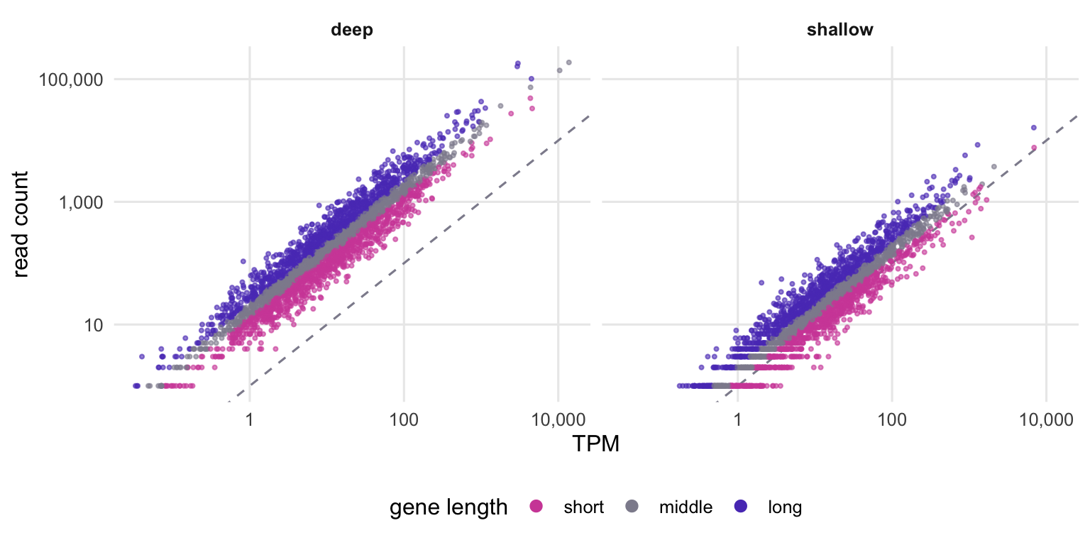
Two scatter plots of read count against TPM on log axes. In the deep panel the points lie well above a dashed diagonal line; in the shallow panel they lie closer to it, with some short genes below it. In both panels the points form three overlapping clouds by gene length, with long genes highest, meaning more reads at the same TPM.
Figure 1: Read count against TPM for every tested gene in one sample of the first simulated experiment, in the deep and in the shallow setting, on log scales. Colour marks the gene length third. The dashed line is where the rounded TPM would equal the count.

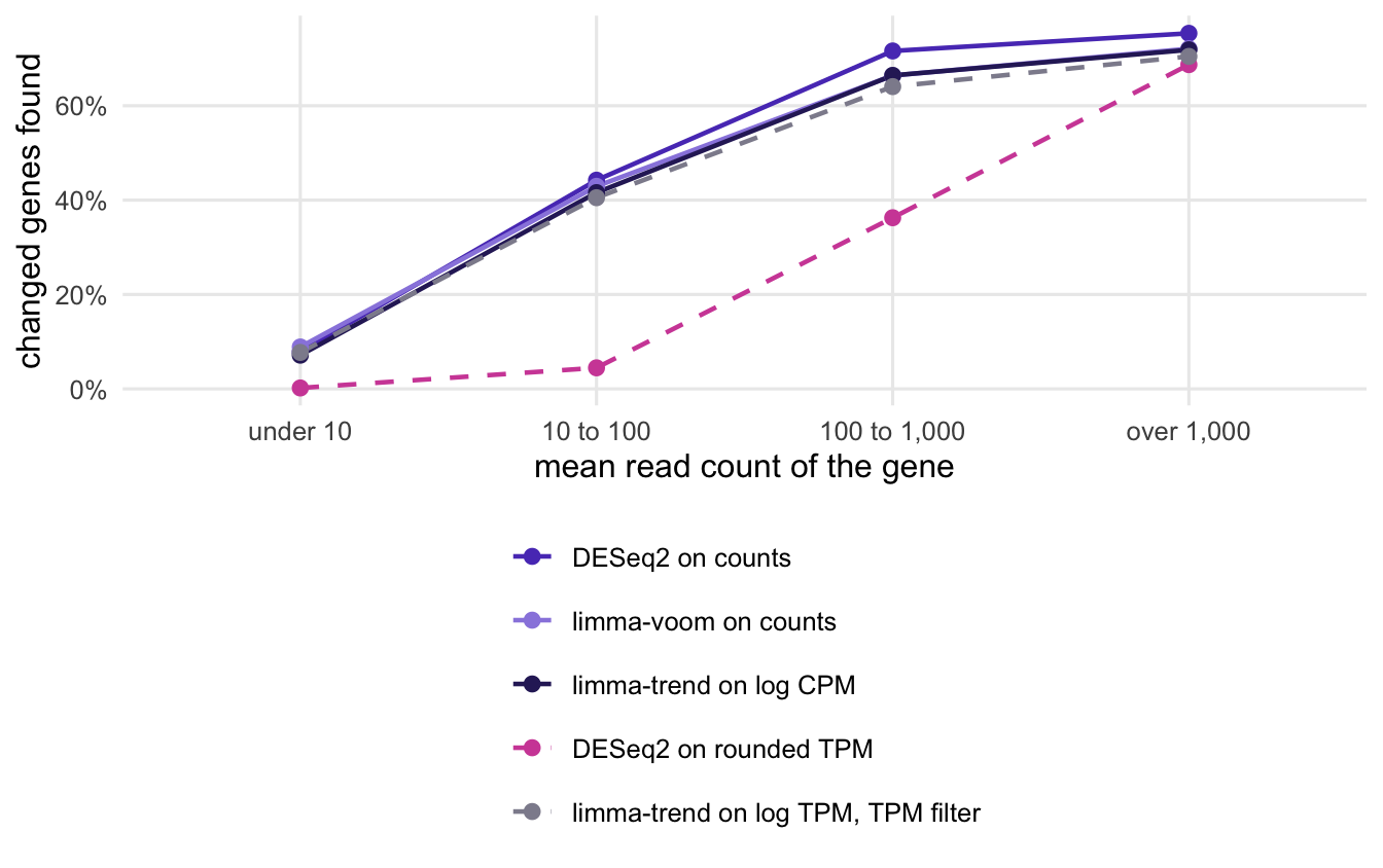
In the deep setting a gene had a median of 16.8 reads per TPM unit in a sample of middle depth. Rounding the TPM and calling it a count tells DESeq2 that each gene was measured with that many times fewer reads than it was. A negative binomial model splits a gene’s variance into counting noise, equal to the mean, and biological variation, which grows with the square of the mean. Dividing a count by a factor divides its variance by the square of that factor, so rounded TPM has much less counting noise than the model assumes for values of its size. The model overstates the noise and the test loses power, most of all where counting noise dominates, at low expression. Among genes with 10 to 100 reads, DESeq2 found 4% of the changed genes from rounded TPM and 44% from the counts (next figure). Rounding also turned 5.2% of the non-zero counts into zeros.

arms <- c("deseq_counts", "voom_counts", "trend_cpm", "deseq_tpm", "trend_tpm")
d <- expand.grid(method = arms, bin = names(bins), stringsAsFactors = FALSE)
d$power <- mapply(function(m, k) sp("deep", m, k), d$method, d$bin)
d$bin <- factor(bins[d$bin], levels = bins)
d$method <- factor(d$method, levels = arms)
d$input <- on_tpm(as.character(d$method))
ggplot(d, aes(bin, power, colour = method, linetype = input, group = method)) +
  geom_line(linewidth = 0.8) +
  geom_point(size = 2.2) +
  scale_colour_manual(values = method_col, labels = method_lab, name = NULL) +
  scale_linetype_manual(values = c(counts = "solid", TPM = "dashed"), guide = "none") +
  scale_y_continuous(labels = function(x) paste0(100 * x, "%")) +
  labs(x = "mean read count of the gene", y = "changed genes found") +
  guides(colour = guide_legend(ncol = 1, override.aes = list(
    linetype = ifelse(on_tpm(arms) == "TPM", "dashed", "solid")))) +
  theme_pc
Line chart of the share of changed genes found against four mean-count bins. Three solid lines for the analyses of counts and a dashed line for limma-trend on log TPM rise together from under a tenth in the lowest bin to over 70% in the highest. The dashed line for DESeq2 on rounded TPM stays near zero in the two lower bins and below the others in the two upper bins.
Figure 2: Share of truly changed genes found by each analysis, by the gene’s mean read count, in the deep setting. Genes are pooled over the simulated experiments. Solid lines use the counts, dashed lines the TPM table.

In the shallow setting a gene had a median of 1.7 reads per TPM unit, and the loss of power was smaller: 24% of the changed genes found against 30%. The formula says the error can also run the other way. For a short gene in a sample with only a few million reads, the TPM can be larger than the count, and the model then sees more reads than there were. That shows up in the false discoveries: among short genes in the shallow setting, the realised FDR of DESeq2 on rounded TPM was 8.1%, against 5.5% on the counts, and among long genes 1.3%. Either way, the precision DESeq2 assigns to a rounded TPM is set by the one-million total, not by your sequencing.

The t-test fails for a different reason

With the BH correction, the Welch t-test on log TPM called 74 genes in all 90 experiments together, out of 27,000 that truly changed. On the log counts per million it called 23. (With equal depths, 33 of the 44 calls on log TPM were false; see the second table below.) Finding almost nothing is not the fault of TPM. With 3 samples per group, each gene’s variance is estimated from almost no data. The Welch test’s degrees of freedom always lie between 2 and 4 with this design, whatever the input (the median was 3.2 on log TPM), so its p-values rarely get small enough to survive a correction over thousands of genes. limma borrows information across genes: on the same log TPM values, its empirical Bayes step added a median of 19.1 prior degrees of freedom to the 4 residual ones in the deep setting. The fix is a moderated test, whatever the input.

Without the correction, the same t-test on log TPM looks productive: it found 58% of the changed genes in the deep setting, but 33% of its calls were false, and in the shallow setting 41%. That is the multiple-testing problem of running thousands of tests at p < 0.05, not a TPM problem.

limma-trend on log TPM

The control comes first: limma-trend on the log counts per million found about as many changed genes as limma-voom in all three settings (57% against 57% deep, 30% against 31% shallow, 31% against 29% with equal depths). So limma-trend itself is not the problem here, even with the 4-fold depth range, a little beyond the guide’s advice. Any difference between limma-trend on counts and on TPM comes from the input.

With deep sequencing the input made little difference: 55% of the changed genes found on log TPM against 57% on log counts per million. With shallow sequencing it did: 21% against 30%, and 21% against 31% with equal depths.

Most of that gap is the filter. At 1.7 reads per TPM unit, the usual filter kept 2,681 of the 3,000 genes on average, where filterByExpr() kept 1,839; the extra genes have almost no reads, add to the multiple-testing burden and pull down the low end of the variance trend. On filterByExpr()’s genes, limma-trend on log TPM found 27% in the shallow setting and 29% with equal depths. No fixed TPM cut-off can be right at both depths, because the reads behind a TPM unit are set by the depth, as the formula shows. Scaling the cut-off with the depth helped only partly (24% and 26%), though it kept about as many genes as filterByExpr() (1,960 on average): the reads behind a TPM unit also depend on the gene’s length, so a TPM cut-off keeps the wrong genes, too many short ones with few reads and too few long ones with plenty.

The length is the second thing TPM hides, and it matters beyond the filter.

arms <- c("deseq_counts", "trend_cpm", "deseq_tpm", "trend_tpm", "trend_tpm_fbe")
thirds <- c("short", "middle", "long")
d <- expand.grid(method = arms, third = thirds, setting = names(settings),
                 quantity = c("found", "FDR"), stringsAsFactors = FALSE)
d$value <- mapply(function(m, k, st, q) if (q == "found") sp(st, m, k) else sf(st, m, k),
                  d$method, d$third, d$setting, d$quantity)
d$third <- factor(d$third, levels = thirds)
d$setting <- factor(settings[d$setting], levels = settings)
d$quantity <- factor(ifelse(d$quantity == "found", "changed genes found", "realised FDR"),
                     levels = c("changed genes found", "realised FDR"))
d$method <- factor(d$method, levels = arms)
d$input <- on_tpm(as.character(d$method))
nominal <- data.frame(quantity = factor("realised FDR", levels = levels(d$quantity)),
                      y = v("fdr_level"))
ggplot(d, aes(third, value, colour = method, linetype = input, group = method)) +
  geom_hline(data = nominal, aes(yintercept = y), linetype = "dotted", colour = "#8e8c9c") +
  geom_line(linewidth = 0.8) +
  geom_point(size = 2) +
  facet_grid(quantity ~ setting, scales = "free_y") +
  scale_colour_manual(values = method_col, labels = method_lab, name = NULL) +
  scale_linetype_manual(values = c(counts = "solid", TPM = "dashed"), guide = "none") +
  scale_y_continuous(labels = function(x) paste0(100 * x, "%")) +
  labs(x = "gene length", y = NULL) +
  guides(colour = guide_legend(ncol = 1, override.aes = list(
    linetype = ifelse(on_tpm(arms) == "TPM", "dashed", "solid")))) +
  theme_pc
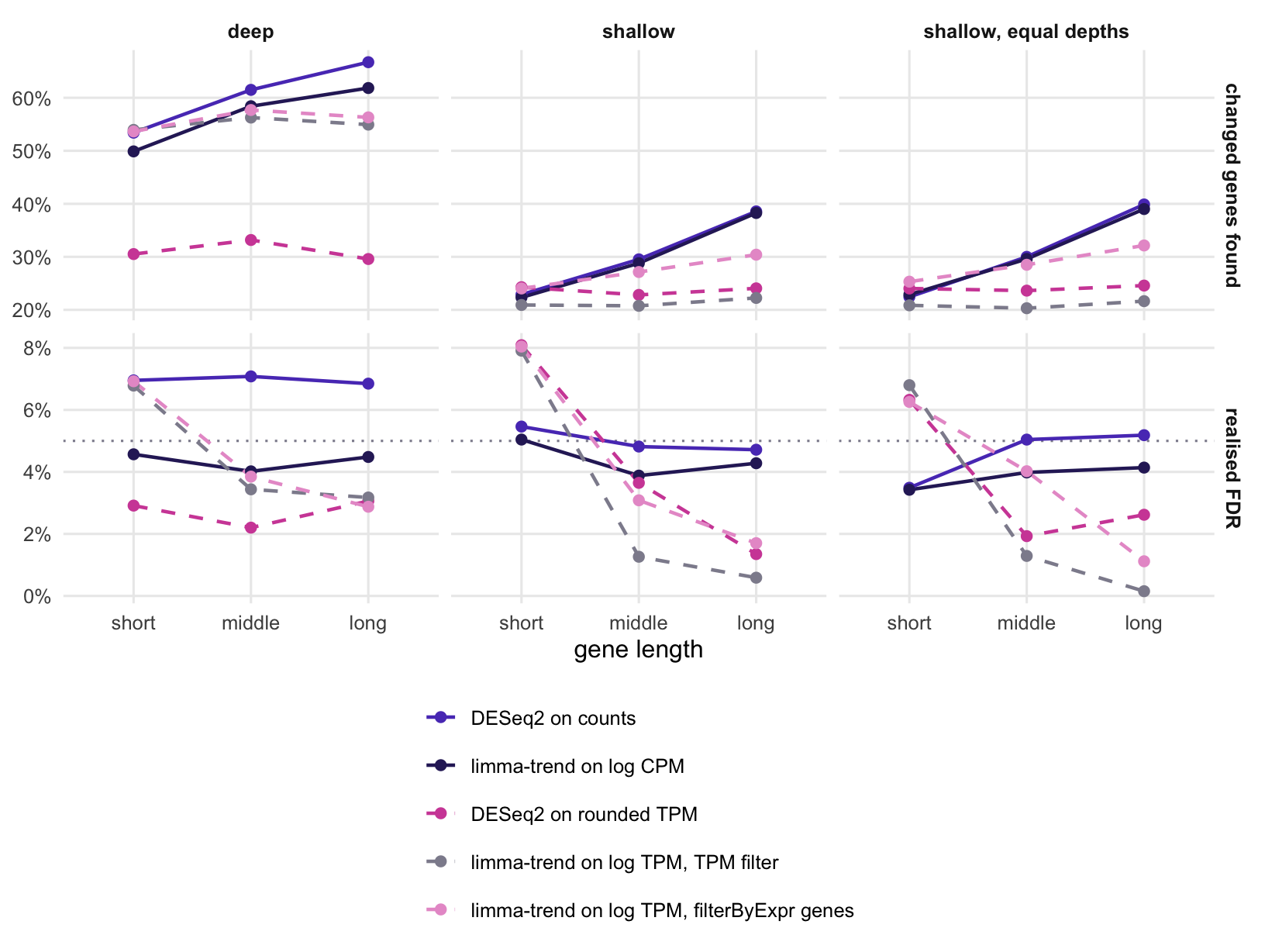
Six panels in two rows, one column per setting. Top row: with counts, the share of changed genes found rises from short to long genes; the dashed TPM lines stay flat or rise less, so they fall behind for long genes, most in the two shallow settings. Bottom row: the solid count lines stay near the dotted nominal line in every length third, while the dashed limma-trend lines on TPM lie above it for short genes and below it for long genes; the dashed DESeq2 line on rounded TPM does the same in the two shallow settings.
Figure 3: Share of truly changed genes found (top) and realised FDR among the calls (bottom), by gene length third, in the three settings. Genes are pooled over the simulated experiments. Solid lines use the counts, dashed lines the TPM table; the dotted line marks the nominal FDR.

With counts, the analyses found more of the changed long genes than of the short ones: a long gene has more reads at the same abundance, so its change is measured more precisely. On the TPM scale that advantage is gone. limma-trend fits one variance trend against the average log TPM, and at a given TPM a long gene has more reads, and less noise, than a short one. The trend gives both the same prior variance: too much for the long gene, too little for the short one. The first costs power, the second false discoveries. In the shallow setting limma-trend on log TPM found 22% of the changed long genes against 38% on log counts per million, and even on filterByExpr()’s genes only 30%. Its realised FDR among short genes was 6.8%, 7.9% and 6.8% in the three settings, and among long genes 3.2%, 0.6% and 0.2%. On the log counts per million the same pipeline stayed between 3.4% and 5.0% in every length third. The overall FDR of limma-trend on TPM, 2.8% to 4.5% across the settings, looks fine only because the two errors partly cancel. With deep sequencing the power side is smaller (55% against 62% for long genes), because at high counts most of a gene’s variance is biological, and dividing by the length leaves that part unchanged on the log scale.

The offset in log2(TPM + 1) matters less. With log2(TPM + 0.1), limma-trend found 54% of the changed genes in the deep setting, about the same as with + 1, and 17% in the shallow one, several points fewer (the post on log2(x + 1) shows what the constant does to low counts).

One reference arm is itself a little off: DESeq2 on the counts had a realised FDR of 6.9% in the deep setting (Monte Carlo standard error 0.3%, from simulating 30 experiments), slightly above the nominal level; a check outside this page, with each experiment fitted separately, gave the same. That is a property of DESeq2 on this simulation, not of TPM; the simulated dispersions do not follow DESeq2’s parametric trend exactly, which may be the reason. All analyses and settings, averaged over the experiments, first the share of changed genes found:

all_arms <- names(method_lab)
tab <- data.frame(analysis = unname(method_lab), check.names = FALSE,
                  sapply(names(settings), function(st) pct(sapply(all_arms, pw, st = st), 1)))
names(tab)[-1] <- settings
knitr::kable(tab, row.names = FALSE, align = "lrrr")
analysis deep shallow shallow, equal depths
DESeq2 on counts 60.5% 30.4% 30.8%
limma-voom on counts 57.2% 30.9% 29.1%
limma-trend on log CPM 56.7% 29.9% 30.6%
DESeq2 on rounded TPM 31.1% 23.7% 24.1%
limma-trend on log TPM, TPM filter 55.0% 21.3% 20.9%
limma-trend on log TPM, filterByExpr genes 55.9% 27.2% 28.7%
limma-trend on log TPM, depth-scaled filter 55.5% 24.0% 25.6%
Welch t-test on log TPM, BH 0.2% 0.1% 0.1%
Welch t-test on log CPM, BH 0.1% 0.1% 0.1%
Welch t-test on log TPM, unadjusted p 58.0% 38.4% 39.5%

and the realised FDR, with its Monte Carlo standard error in brackets. For the two corrected t-tests, which called almost nothing, the table gives the total number of calls over the 30 experiments and how many of them were false instead:

fdr_cell <- function(st, m) {
  if (m %in% c("welch_tpm", "welch_cpm"))
    return(sprintf("%s calls, %s false", num(v("calls_total", st, m)), num(v("false_total", st, m))))
  sprintf("%s (%s)", pct(fd(st, m), 1), pct(v("se_fdr", st, m), 1))
}
tab <- data.frame(analysis = unname(method_lab), check.names = FALSE,
                  sapply(names(settings), function(st) sapply(all_arms, fdr_cell, st = st)))
names(tab)[-1] <- settings
knitr::kable(tab, row.names = FALSE, align = "lrrr")
analysis deep shallow shallow, equal depths
DESeq2 on counts 6.9% (0.3%) 4.9% (0.4%) 4.8% (0.5%)
limma-voom on counts 4.8% (0.3%) 5.3% (0.3%) 3.3% (0.4%)
limma-trend on log CPM 4.3% (0.3%) 4.3% (0.3%) 3.9% (0.4%)
DESeq2 on rounded TPM 2.6% (0.3%) 4.4% (0.5%) 3.7% (0.5%)
limma-trend on log TPM, TPM filter 4.5% (0.3%) 3.1% (0.3%) 2.8% (0.4%)
limma-trend on log TPM, filterByExpr genes 4.5% (0.3%) 4.0% (0.4%) 3.5% (0.4%)
limma-trend on log TPM, depth-scaled filter 4.5% (0.3%) 3.1% (0.4%) 2.9% (0.3%)
Welch t-test on log TPM, BH 22 calls, 1 false 8 calls, 2 false 44 calls, 33 false
Welch t-test on log CPM, BH 7 calls, 1 false 7 calls, 0 false 9 calls, 0 false
Welch t-test on log TPM, unadjusted p 33.3% (0.4%) 41.0% (0.5%) 41.9% (0.5%)

What to do in practice

Get the counts. They usually exist somewhere. If the data are in GEO, look for a raw count matrix among the supplementary files. For human RNA-seq runs NCBI also computes raw counts from the submitted reads (its page announced mouse to follow) and offers them on the series page as NCBI-generated RNA-seq count data; the same page describes its TPM and FPKM tables as “suitable input for qualitative analysis and visualizing gene expression abundance”, and the raw counts as suitable “for differential expression analysis tools like DESeq2, edgeR or limma voom”.

If a colleague ran Salmon, kallisto or RSEM, ask for the quantification files and import them with tximport (Soneson, Love and Robinson 2015). DESeqDataSetFromTximport() takes the estimated counts and uses the average transcript lengths as an offset. For limma-voom or edgeR, the tximport vignette describes a second route: countsFromAbundance = "lengthScaledTPM" returns count-scale values that you use “directly as you would a regular count matrix”. edgeR 4.10 and later also offer DGEListFromTximport(), which keeps the estimated counts and stores the lengths as an offset. If the pipeline was featureCounts or htseq-count, the counts are its output.

If a TPM table really is all you have, do not round it into DESeq2, and do not run a t-test with a handful of samples, with or without a correction. limma-trend on log TPM was the least bad option here, with two cautions. Filter with care: if the total number of reads per sample is reported, convert a count threshold into TPM with it rather than using a fixed TPM cut-off, and know that it still ignores gene length. And read the gene list with its bias in mind: expect a few too many false calls among short genes and missed changes among long genes, most of all in shallowly sequenced data.

# from Salmon (or kallisto, RSEM) output: estimated counts plus a length offset
library(tximport)
txi <- tximport(files, type = "salmon", tx2gene = tx2gene)
dds <- DESeqDataSetFromTximport(txi, samples, ~ condition)
dds <- DESeq(dds)

# for limma-voom or edgeR: count-scale values, no offset
txi_ls <- tximport(files, type = "salmon", tx2gene = tx2gene,
                   countsFromAbundance = "lengthScaledTPM")
y <- DGEList(txi_ls$counts)          # then filterByExpr(), normLibSizes(), voom() as usual

# only a TPM table: limma-trend on log2(TPM + 1)
reads_m <- median(total_reads) / 1e6       # reads per sample in millions, if reported
keep <- rowSums(tpm >= 10 / reads_m) >= 3  # about 10 reads in at least 3 samples
fit <- lmFit(log2(tpm[keep, ] + 1), design)
fit <- eBayes(fit, trend = TRUE)
topTable(fit, coef = 2)

References

Wagner GP, Kin K, Lynch VJ 2012 Theory in Biosciences 131(4):281-285 (doi:10.1007/s12064-012-0162-3)

Zhao S, Ye Z, Stanton R 2020 RNA 26(8):903-909 (doi:10.1261/rna.074922.120)

Love MI, Huber W, Anders S 2014 Genome Biology 15(12):550 (doi:10.1186/s13059-014-0550-8)

Law CW, Chen Y, Shi W et al. 2014 Genome Biology 15(2):R29 (doi:10.1186/gb-2014-15-2-r29)

Soneson C, Love MI, Robinson MD 2015 F1000Research 4:1521 (doi:10.12688/f1000research.7563.1)

The numbers on this page were computed with the versions below.

R version 4.5.3 (2026-03-11)
Bioconductor 3.22
Biobase 2.70.0, BiocGenerics 0.56.0, DESeq2 1.50.2, edgeR 4.8.2,
generics 0.1.4, GenomicRanges 1.62.1, ggplot2 4.0.3, IRanges 2.44.0,
limma 3.66.0, MatrixGenerics 1.22.0, matrixStats 1.5.0, S4Vectors
0.48.1, Seqinfo 1.0.0, SummarizedExperiment 1.40.0