Adding 1 before log2 shrinks the fold changes of low-count genes by an amount set by expression and by the constant. A simulation against DESeq2 and edgeR.
You have a table of counts, you want a fold change, and the zeros get in the way: log2(0) is minus infinity. So you add 1, take log2(count + 1), average each group and subtract. This is a very common shortcut in RNA-seq analysis, and the question behind it is simple: what does the added 1 do to the fold change?
The short answer: it pulls the fold changes of low-count genes towards zero, by an amount that depends on how many reads the gene has and on the constant you picked, not on how many samples you have. In the simulation below, genes whose true log2 fold change is 2 (a four-fold change) and whose mean count is between 2 and 5 reads come out at a median of 1.44 with log2(count + 1). Measuring more samples does not fix it.
The setup
The simulation is deliberately plain. Each gene gets a mean count drawn on a log scale between half a read and a thousand reads, so every expression level is well represented. Most genes do not change; the rest go up or down by exactly a log2 fold change of 2. Counts are drawn from a negative binomial distribution, which is the usual model for RNA-seq counts: Poisson-like sampling noise plus biological variation between samples, set here by a dispersion parameter. The six samples differ a little in sequencing depth.
n_genes <-4000; n_rep <-3; disp_sim <-0.1; true_abs <-2; p_de <-0.3simulate_counts <-function(G = n_genes, n = n_rep, disp = disp_sim) { mu <-exp(runif(G, log(0.5), log(1000))) # mean count of each gene lfc <-sample(c(0, true_abs, -true_abs), G, replace =TRUE, # true log2 FC, B vs Aprob =c(1- p_de, p_de /2, p_de /2)) muA <-2* mu / (1+2^lfc) # the two group means average to mu muB <- muA *2^lfc sf <-rep_len(c(0.8, 1.0, 1.2, 0.9, 1.1, 1.0), 2* n) # sequencing depth M <-cbind(matrix(muA, G, n), matrix(muB, G, n)) *rep(sf, each = G) counts <-matrix(rnbinom(length(M), mu = M, size =1/ disp), G,dimnames =list(paste0("g", 1:G), paste0("s", 1:(2* n))))storage.mode(counts) <-"integer"list(counts = counts, group =factor(rep(c("A", "B"), each = n)),mu = mu, lfc = lfc)}# mean-count bins used to summarise the resultsbrk <-c(0.5, 2, 5, 10, 30, 100, 1000)bin_lab <-c("0.5-2", "2-5", "5-10", "10-30", "30-100", "100-1000")set.seed(20260825)sim <-simulate_counts()n_de <-sum(sim$lfc !=0)
That gives 4,000 genes in 3 versus 3 samples, of which 1,142 truly change. A few things to keep in mind. The dispersion is the same for every gene (0.1); real data usually have more biological variation at low counts. That makes low-count estimates noisier, and, as the exact calculation further down shows, it makes the shortcut’s problem larger, not smaller. Every changed gene changes by the same amount, and the attenuation grows with the size of the true change. The share of unchanged genes (70%) sets how hard apeglm shrinks, so the error comparison near the end depends on it. Finally, genes are grouped by their true mean count, which we know because we simulated it; with real data the closest thing is DESeq2’s baseMean column.
The shortcut: add a constant, then log
Here is the shortcut, on counts normalised for sequencing depth with DESeq2’s size factors. The second version is the edgeR equivalent, log counts per million from cpm(log = TRUE).
A <- sim$group =="A"; B <- sim$group =="B"dds <-DESeqDataSetFromMatrix(sim$counts, data.frame(group = sim$group), ~ group)dds <-estimateSizeFactors(dds)norm_counts <-counts(dds, normalized =TRUE)# the common shortcut: log2(count + c), then difference of group meansnaive_lfc <-function(x, c) rowMeans(log2(x[, B] + c)) -rowMeans(log2(x[, A] + c))lfc_plus1 <-naive_lfc(norm_counts, 1)# edgeR log-CPM with its default prior.county_all <-normLibSizes(DGEList(sim$counts, group = sim$group))logcpm <-cpm(y_all, log =TRUE)lfc_logcpm <-rowMeans(logcpm[, B]) -rowMeans(logcpm[, A])prior_default <-formals(edgeR:::cpm.DGEList)$prior.count# a noise-free example: 1 read versus 4 readsex_plus1 <-log2((4+1) / (1+1))
Why should adding 1 matter? For a gene with thousands of reads it does not: 1 is nothing next to 2,000. For a gene with a handful of reads it is a large part of the value. A gene with exactly 1 read in one group and 4 in the other has a true log2 fold change of 2, but log2(4 + 1) - log2(1 + 1) is 1.32. The constant is added to both groups, so the ratio is dragged towards 1 and its logarithm towards 0.
The edgeR version adds a constant too. cpm(..., log = TRUE) has a default prior.count of 2, and its help page says this count is scaled in proportion to library size, so a sample of average depth gets 2 reads added before the log. That is more than 1, so expect more attenuation, not less.
Model-based estimates
The alternative is to estimate the fold change inside a count model. DESeq2 fits a negative binomial generalised linear model per gene (Love et al. 2014); since version 1.16, results() reports the maximum likelihood estimate (MLE) of the log2 fold change without shrinkage, according to the DESeq2 vignette. lfcShrink() then adds a shrunken estimate.
dds <-DESeq(dds, quiet =TRUE)res <-results(dds, name ="group_B_vs_A") # maximum likelihood LFCshr <-lfcShrink(dds, coef ="group_B_vs_A", type ="apeglm", quiet =TRUE)shrink_default <-eval(formals(DESeq2::lfcShrink)$type)[1]
The default type of lfcShrink() is apeglm, the method used here.
For edgeR the recommended route is the quasi-likelihood pipeline (Chen et al. 2016). In the edgeR QL workflow used here, filterByExpr() removes genes with too few reads, then the data are normalised, dispersions are estimated, and glmQLFit() and glmQLFTest() do the testing. glmQLFit() is called with legacy = FALSE, the quasi-likelihood method that is the default from edgeR 4.2 onwards; the edgeR in this container is older, so the argument is set explicitly. glmQLFit() fits its coefficients through glmFit(), which adds a small prior count of 0.125 to each count (scaled to library size) before fitting, so the logFC column is lightly shrunk. predFC() computes the same kind of estimate directly.
design <-model.matrix(~ group, data =data.frame(group = sim$group))keep <-filterByExpr(y_all, group = sim$group)y <-normLibSizes(y_all[keep, , keep.lib.sizes =FALSE])y <-estimateDisp(y, design)fit <-glmQLFit(y, design, legacy =FALSE)qlf <-glmQLFTest(fit, coef =2)# predFC on every gene (no filtering), to see the whole expression rangey_pf <-estimateDisp(y_all, design)lfc_predfc <-predFC(y_pf, design)[, 2]predfc_default <-formals(edgeR:::predFC.DGEList)$prior.countglmfit_default <-formals(edgeR:::glmFit.DGEList)$prior.countql_vs_predfc <-max(abs(qlf$table$logFC -predFC(y, design)[, 2]))kept_bin <-tapply(keep, cut(sim$mu, brk, labels = bin_lab, include.lowest =TRUE), mean)
The check agrees: the default prior count is 0.125 in predFC() and 0.125 in glmFit(), and on the filtered genes the glmQLFTest() fold changes and predFC() differ by at most 0.0022. The filtering step matters here too. In this data set filterByExpr() keeps 0% of the genes with a mean count below 2, 0% of those between 2 and 5 and 21% of those between 5 and 10. So edgeR’s standard pipeline never reports a fold change for most of the genes where the pseudocount problem lives. To look at the whole range anyway, the comparison uses predFC() on all genes.
What happens by expression level
est <-data.frame(mu = sim$mu, lfc = sim$lfc,bin =cut(sim$mu, brk, labels = bin_lab, include.lowest =TRUE),plus1 = lfc_plus1, logcpm = lfc_logcpm, predfc = lfc_predfc,mle = res$log2FoldChange, apeglm = shr$log2FoldChange)# genes with no reads in any sample carry no information; DESeq2 gives them no LFCall_zero <-rowSums(sim$counts) ==0n_all_zero <-sum(all_zero); stopifnot(all(is.na(est$mle) == all_zero))est <- est[!all_zero, ]methods <-c(plus1 ="log2(count + 1)", logcpm ="edgeR logCPM",predfc ="edgeR predFC", mle ="DESeq2 MLE", apeglm ="DESeq2 apeglm")de <- est[est$lfc !=0, ]# median estimate for genes whose true LFC is +2 or -2 (sign flipped so truth is +2)med <-sapply(names(methods), function(m) tapply(de[[m]] *sign(de$lfc), de$bin, median))rmse <-sapply(names(methods), function(m)tapply((est[[m]] - est$lfc)^2, est$bin, function(v) sqrt(mean(v))))n_bin_de <-table(de$bin)stopifnot(isTRUE(all.equal(headline, unname(med["2-5", "plus1"]))))# a pseudocount added to the group MEAN instead of to each sample before the lognc <- norm_counts[!all_zero, ]group_mean_lfc <-function(c) log2(rowMeans(nc[, B]) + c) -log2(rowMeans(nc[, A]) + c)is_low <- est$lfc !=0& est$bin =="0.5-2"gm_low <-sapply(c(0.125, 1), function(c)median((group_mean_lfc(c) *sign(est$lfc))[is_low]))
Genes with no reads in any sample (14 of them) are dropped, since DESeq2 reports no fold change for them and no method can say anything about them. For the truly changed genes, the sign of the down-regulated ones is flipped so that the right answer is always 2, and each bin gets the median estimate. The bin with the fewest changed genes still holds 109 changed genes.
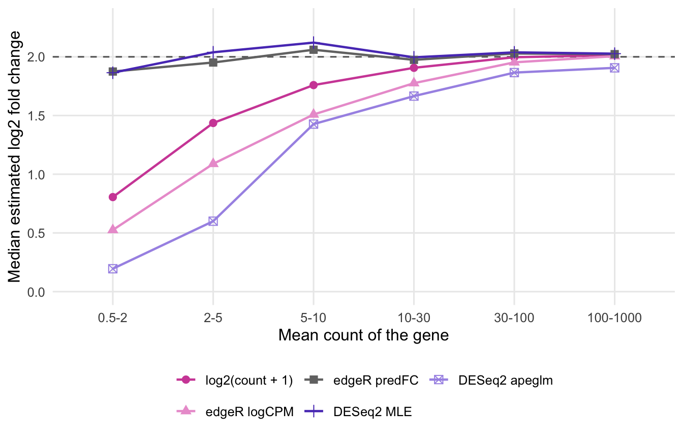
Figure 1: Median estimated log2 fold change of genes whose true log2 fold change is 2 (dashed line), by the mean count of the gene. The same simulated data set, five ways of computing the fold change.
DESeq2’s MLE and edgeR’s predFC() stay near the truth in every bin: 1.86 and 1.87 in the lowest bin, where genes have fewer than 2 reads on average. The shortcut does not. With log2(count + 1) the median is 0.81 in that bin, 1.44 between 2 and 5 reads and 1.76 between 5 and 10, and it only reaches 1.91 for genes with 10 to 30 reads. The edgeR log-CPM version, with its larger constant, is lower at every low-count bin: 0.52, 1.09 and 1.51 in the first three. Above 100 reads the methods agree (2.01 to 2.03).
The same true fold change is therefore reported as small or large depending on how many reads the gene has. A lowly expressed transcription factor and a highly expressed structural gene that both quadruple will not look alike in the table.
edgeR’s estimate is not free of a pseudocount either. It adds one, but a small one (0.125), and the log is taken of a fitted group mean rather than averaged over individual samples. You can mimic that without a model: taking log2(group mean + c) on the normalised counts gives a median of 1.83 in the lowest bin with c = 0.125, but 0.87 with c = 1. So what matters is the size of the constant next to the counts, not whether a pseudocount is used at all.
The constant decides the answer
The size of the attenuation is set by the constant and the count level, not by the number of samples. This can be computed exactly, without simulation. With unlimited replicates, the average of log2(count + c) in each group converges to its expected value under the negative binomial distribution (for samples of equal depth), and that expectation is a sum over all possible counts.
# Expected value of log2(X + c) for a negative binomial X, summed over its distributionelog <-function(m, c, disp) { x <-0:qnbinom(1-1e-10, mu = m, size =1/ disp)sum(dnbinom(x, mu = m, size =1/ disp) *log2(x + c))}# what mean(log2(B + c)) - mean(log2(A + c)) converges to with unlimited replicatesexpected_lfc <-function(mu, c, true_lfc = true_abs, disp = disp_sim) { muA <-2* mu / (1+2^true_lfc); muB <- muA *2^true_lfcelog(muB, c, disp) -elog(muA, c, disp)}mu_grid <-exp(seq(log(0.5), log(1000), length.out =120))c_values <-c(0.1, 0.5, 1, 2, 5)exact <-expand.grid(mu = mu_grid, c = c_values)exact$lfc <-mapply(expected_lfc, exact$mu, exact$c)# the mean count at which the expected estimate comes within 0.1 of the truthtol <-0.1mu_within <-function(c, true_lfc = true_abs, disp = disp_sim)uniroot(function(m) expected_lfc(m, c, true_lfc, disp) - (true_lfc - tol), c(0.5, 1e4))$rootmu_ok_plus1 <-mu_within(1)mu_ok_plus5 <-mu_within(5)lfc_big <-4mu_ok_big <-mu_within(1, true_lfc = lfc_big) # a larger true changemax_c01 <-max(exact$lfc[exact$c ==0.1])mu_max_c01 <- exact$mu[exact$c ==0.1][which.max(exact$lfc[exact$c ==0.1])]# more biological variation: same gene (mean 3 reads, c = 1), higher dispersiondisp_hi <-0.5; mu_ex <-3att_base <-expected_lfc(mu_ex, 1)att_hi <-expected_lfc(mu_ex, 1, disp = disp_hi)mu_ok_disp <-mu_within(1, disp = disp_hi)# the exact value for the simulated changed genes in the two lowest bins (median per bin)exact_bin <-sapply(c("0.5-2", "2-5"), function(b)median(sapply(de$mu[de$bin == b], expected_lfc, c =1)))
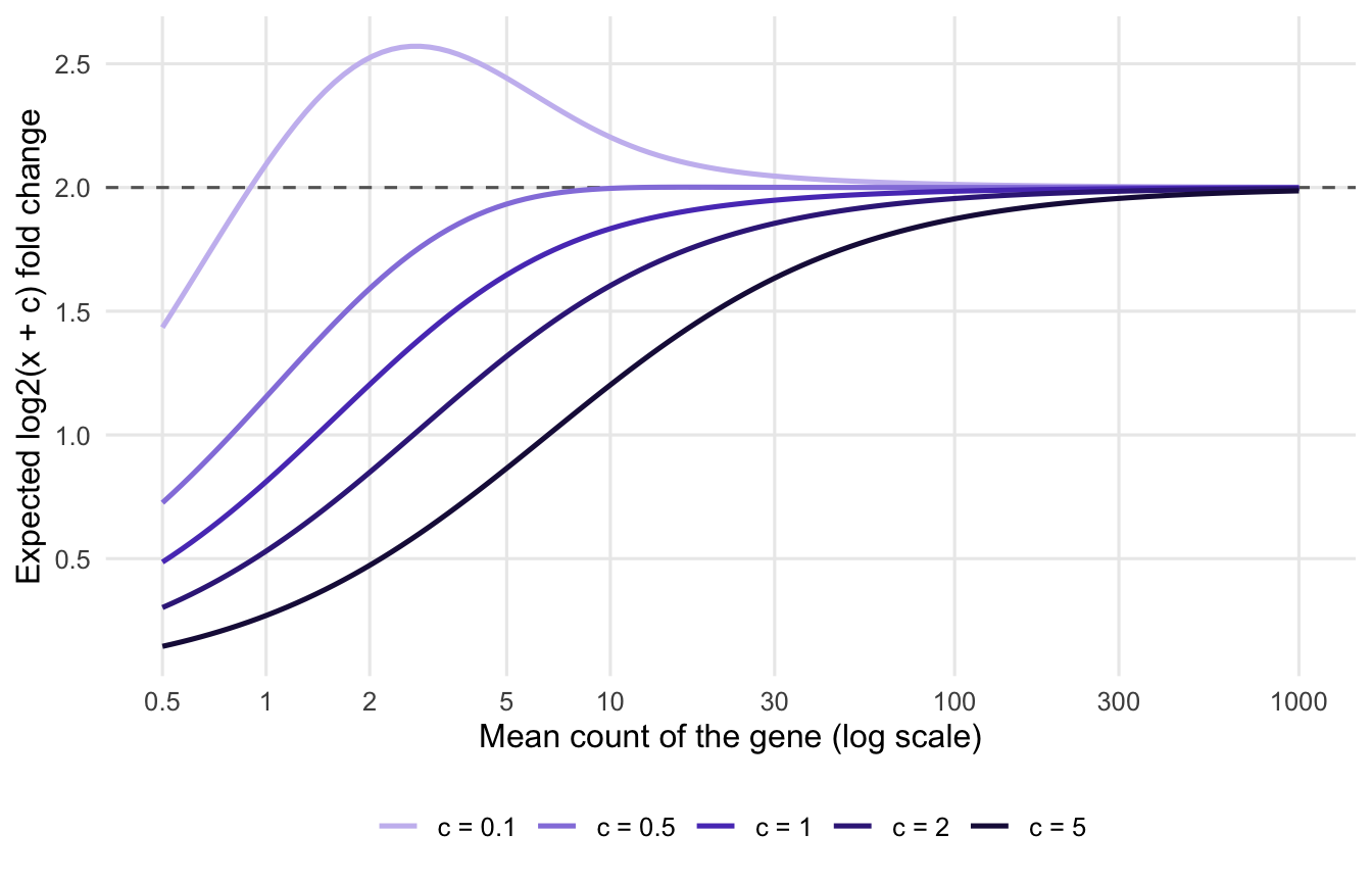
Figure 2: What the pseudocount estimator converges to with unlimited replicates, for a gene with a true log2 fold change of 2 (dashed line), as a function of its mean count and of the pseudocount c. Computed exactly from the negative binomial distribution, no simulation.
With c = 1, the expected estimate comes within 0.1 of the true value only once the gene averages about 16 reads. With c = 5 that point moves out to about 128 reads. A small constant fails in the other direction: with c = 0.1 a zero becomes log2(0.1), about -3.3, so a group with a few zeros is pushed far down, and the expected estimate overshoots to 2.57 for genes averaging about 2.8 reads. Between those choices you can get almost any answer for a low-count gene.
These are two different failures. A constant that is large next to the counts attenuates the fold change. A tiny constant added to each sample before averaging the logs turns every zero into a large negative number and inflates it. Adding the constant to a group mean, as edgeR does in effect, avoids most of the second problem: a single zero no longer drags the group down, and only a group with no reads in any of its samples still does.
More biological variation makes it worse. For a gene averaging 3 reads with c = 1, the expected estimate is 1.42 at the simulated dispersion of 0.1 and 1.29 at a dispersion of 0.5.
Because the mean count is expression multiplied by sequencing depth, the same gene in the same biology also gets a different fold change from log2(count + 1) when it is sequenced deeper. Nothing about the gene has changed; only the constant has become smaller relative to its counts.
Is shrinkage itself the problem?
Look again at the first figure. DESeq2’s apeglm estimate is pulled towards zero even harder than the shortcut: 0.19 in the lowest bin and 0.60 between 2 and 5 reads. So a fair question is whether shrinking low-count fold changes is bad at all.
It is not bad in itself. With a handful of reads and 3 samples per group, the MLE is noisy, and pulling noisy estimates towards zero reduces the typical error. Measured as root mean squared error over all genes in the lowest bin (changed and unchanged together), the MLE is off by 1.30, log2(count + 1) by 0.87 and apeglm by 0.95. In that bin the shortcut is actually the most accurate of the three on this measure. Above 100 reads the order changes and apeglm has the smallest error (0.36, against 0.40 for the MLE).
The difference is where the shrinkage comes from. apeglm places a heavy-tailed prior on the fold changes, estimated from all genes, and combines it with each gene’s likelihood (Zhu et al. 2019). When a gene carries more information, the likelihood dominates and the shrinkage fades. The pseudocount has no such link to information: its pull depends only on the count level and the constant. Adding replicates separates the two.
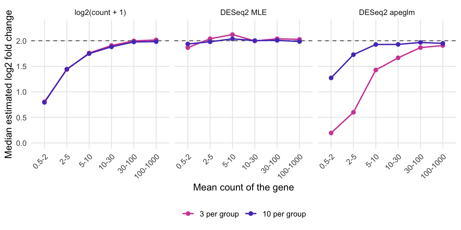
Figure 3: Median estimated log2 fold change of truly changed genes (true value 2, dashed line) with 3 and with 10 samples per group, for the pseudocount shortcut and the two DESeq2 estimates.
With 10 samples per group instead of 3, the apeglm median in the lowest bin rises from 0.19 to 1.27, and between 2 and 5 reads from 0.60 to 1.73. The MLE stays near the truth in both (1.94 in the lowest bin with 10 samples). The pseudocount shortcut does not move: 0.81 becomes 0.79 and 1.44 becomes 1.44. That is the signature of a bias rather than of noise control. More data makes the estimate more precise, but precise about the wrong number: the exact expected value from the previous section, taken as the median over the changed genes of the first data set, is 0.79 for the lowest bin and 1.44 for the next one.
What to do in practice
For reporting an effect size, in a results table, a volcano plot or a sentence such as “gene X is up four-fold”, take the fold change from the count model, not from averaged log values. In DESeq2 that is the log2FoldChange from results(), reported with lfcSE (its standard error) or a confidence interval, because at a few reads per sample it is close to unbiased but very noisy. The alternative is the lfcShrink() value, which the DESeq2 vignette describes as useful for visualisation and ranking. Say which one you report, because for low-count genes with few replicates they differ a lot. In edgeR it is the logFC column from glmQLFTest() after filterByExpr(), which simply does not report the genes with the fewest reads.
A pseudocount is fine where no effect size is being read off. Heatmaps, PCA, clustering and sample-to-sample distances need values on a log-like scale without minus infinity, and there log2(count + 1) does its job. DESeq2 itself provides normTransform(), which adds 1 by default, and the edgeR help page for cpm() describes CPM values as descriptive measures of expression level. For those tasks DESeq2’s vst() and rlog() are usually better still, since they also deal with the high variance of log counts at low expression, as the vignette explains.
If all you have is a table of log2(x + 1) values, for example from a collaborator or a public supplement, treat fold changes of weakly expressed genes as underestimates of unknown size, and do not compare fold changes between genes with very different expression. How weak is weak depends on the gene. In this simulation the estimate comes within 0.1 of the truth only above about 16 reads, and that is the lower end: for a true log2 fold change of 4 the threshold is about 66 reads, and at a dispersion of 0.5 it is about 28. Also check the units of the table. What matters is the value in the table’s own units next to the constant, so for log2(TPM + 1) or log2(CPM + 1) a value of a few TPM or CPM is the danger zone whatever the read count, and sequencing deeper does not help there. If the constant was much smaller than 1 (0.1 in the second figure), the error can go the other way.