Why a Poisson GLM calls false positives on RNA-seq counts with biological replicates, how to spot overdispersion, and what a negative binomial model fixes.
Author
Pseudocount
Published
25 September 2026
Setup: packages and helper functions
suppressPackageStartupMessages({library(edgeR)library(DESeq2)library(ggplot2)})stopifnot(packageVersion("edgeR") >="4.0.0", # normLibSizes() and glmQLFit(legacy = FALSE)packageVersion("limma") >="3.50",packageVersion("DESeq2") >="1.36",packageVersion("ggplot2") >="3.4.0")pct <-function(x, d =1) sprintf(paste0("%.", d, "f%%"), 100* x)num <-function(x) format(x, big.mark =",", scientific =FALSE, trim =TRUE)dec <-function(x, d =2) sprintf(paste0("%.", d, "f"), x)rng <-function(x) paste(pct(min(x)), "to", pct(max(x)))# Poisson and quasi-Poisson likelihood ratio tests for a two-group design, all genes at once.# With a log link, an offset and one mean per group, the fitted values have a closed form:# the group total divided by the group's summed library sizes, times each sample's library size.pois_tests <-function(counts, group, lib) { n <-ncol(counts) fit_null <-outer(rowSums(counts) /sum(lib), lib) fit_full <- countsfor (g inlevels(group)) { j <- group == g fit_full[, j] <-outer(rowSums(counts[, j, drop =FALSE]) /sum(lib[j]), lib[j]) } dev <-function(mu) 2*rowSums(ifelse(counts >0, counts *log(counts / mu), 0) - (counts - mu)) lr <-dev(fit_null) -dev(fit_full) # deviance explained by the group df_res <- n -nlevels(group) pearson <-rowSums(ifelse(fit_full >0, (counts - fit_full)^2/ fit_full, 0)) disp <- pearson / df_res # Pearson dispersion statisticdata.frame(lr = lr,p_pois =pchisq(lr, 1, lower.tail =FALSE), # Poisson: dispersion fixed at 1p_qp =pf(lr / disp, 1, df_res, lower.tail =FALSE), # quasi-Poisson F testpearson = pearson, disp = disp)}# what we can measure because the truth is known# BH is applied to every method's raw p-values in the same way; a missing p-value (DESeq2 can# set one for a count outlier) is counted as not significantscore <-function(p, is_de) { p[is.na(p)] <-1 padj <-p.adjust(p, "BH") call <- padj <0.05list(null_p05 =mean(p[!is_de] <0.05), n_call =sum(call),fdp =if (any(call)) mean(!is_de[call]) else0, power =mean(call[is_de]))}theme_pc <-theme_minimal(base_size =12) +theme(panel.grid.minor =element_blank(), legend.position ="bottom",plot.background =element_rect(fill ="white", colour ="white"))
Why not test RNA-seq counts with a Poisson model? Counts of reads are counts, and the Poisson distribution is the textbook model for counts, so a Poisson regression per gene looks like the obvious test. The problem is that the Poisson model fixes the variance to be equal to the mean, and counts from biological replicates vary far more than that. In the simulation below, a Poisson test gives p < 0.05 for 52.9% of the genes that did not change, and 81.4% of the genes it calls at a 5% false discovery rate are false. A negative binomial test from edgeR on the same data gives 5.3% and 4.6%.
This post shows where the Poisson test goes wrong, two quick diagnostics that catch the problem on your own data, and why the quasi-Poisson model, the usual textbook repair, fixes the false positives but finds less than half as many of the changed genes as a negative binomial test.
Two models for the same counts
Take one gene measured in several mice from the same group. Even with perfect sequencing, the gene’s true expression differs from mouse to mouse. The read count you see has two layers of variation: the biological differences between mice, and the sampling of reads from each library.
The Poisson distribution describes only the second layer. If a library contains a gene at an expected count of , the count has variance . That is a good model for technical replicates, the same library sequenced on several lanes (Marioni et al. 2008), but not for biological ones.
The negative binomial distribution adds the first layer. Its variance is , where is the dispersion: the squared coefficient of variation of the true expression between replicates. This is the model behind edgeR (Robinson, McCarthy and Smyth 2010; McCarthy, Chen and Smyth 2012) and DESeq2 (Love, Huber and Anders 2014). The ratio of the two variances is , so the gap grows with expression. For a gene with a modest dispersion of 0.05 and a mean count of 150, the real variance is 8.5 times the Poisson variance.
The setup
Each gene gets a baseline mean count between a few reads and several thousand, and a dispersion that falls with expression and scatters between genes. There are 4 biological replicates per condition, and 10% of the 3,000 genes truly change by a factor of two, up or down. The rest are null. Sequencing depth differs between samples.
All four analyses below start from the same filtered table: the edgeR recipe of filterByExpr() to drop genes with too few reads to test, then normLibSizes() for TMM normalisation. The Poisson, quasi-Poisson and edgeR fits use the same normalised library sizes as offsets (an offset is a per-sample adjustment for sequencing depth that the model takes as given), so between them only the variance differs. DESeq2 runs its standard workflow on the same genes and estimates its own size factors, and it tests with a Wald test rather than a likelihood ratio or F test.
design <-model.matrix(~ group)y <-DGEList(counts, group = group)keep <-filterByExpr(y, design)y <-normLibSizes(y[keep, , keep.lib.sizes =FALSE])is_de_k <- is_de[keep]lib <-getNormLibSizes(y) # library size x TMM factor# Poisson and quasi-Poisson GLM, one per gene (closed form, checked against glm() below)pt <-pois_tests(y$counts, group, lib)# edgeR quasi-likelihood pipeline: negative binomial GLM + empirical Bayes QL dispersionfit <-glmQLFit(y, design, legacy =FALSE)p_ql <-glmQLFTest(fit, coef =2)$table$PValue# DESeq2 standard workflow on the same genesdds <-DESeqDataSetFromMatrix(y$counts, data.frame(group = group), ~ group)p_deseq <-results(DESeq(dds, quiet =TRUE))$pvalues_pois <-score(pt$p_pois, is_de_k)s_qp <-score(pt$p_qp, is_de_k)s_ql <-score(p_ql, is_de_k)s_deseq <-score(p_deseq, is_de_k)n_kept <-sum(keep)df_prior <- fit$df.priordf_gene <-ncol(counts) -ncol(design)crit_known <-qchisq(0.95, 1) # 5% cut-off with the variance knowncrit_qp <-qf(0.95, 1, df_gene) # quasi-Poisson: variance from df_gene dfcrit_ql <-qf(0.95, 1, df_gene + df_prior) # edgeR QL: plus the prior df
A loop of glm() calls, one per gene, is how most people would write the Poisson test, and it is slow for thousands of genes. With two groups and a log link (the model works on the log of the expected count) the fitted values have a closed form, a direct formula with no iterative fitting, so the helper pois_tests() in the setup chunk computes the same likelihood ratio tests for all genes at once. The next chunk checks it against glm() and anova() on the first 200 genes.
n_check <-200off <-log(lib)p_glm <-t(sapply(seq_len(n_check), function(i) { k <- y$counts[i, ] f_p <-glm(k ~ group +offset(off), family = poisson) f_q <-glm(k ~ group +offset(off), family = quasipoisson)c(anova(f_p, test ="Chisq")[2, "Pr(>Chi)"], anova(f_q, test ="F")[2, "Pr(>F)"])}))max_diff <-max(abs(p_glm -as.matrix(pt[seq_len(n_check), c("p_pois", "p_qp")])))stopifnot(max_diff <1e-4)
Across those genes the largest difference in p-value between the two routes is 6.6e-06.
The Poisson test calls 1,588 genes at 5% FDR. It finds nearly every changed gene, 98.7% of them, but 81.4% of its calls are false. The model assumes that each count varies only by the sampling of reads, so ordinary differences between mice in the same group look to it like a treatment effect. Both negative binomial tools keep the share of null genes below 0.05 close to the promised 5%. DESeq2’s share of false calls, 8.1%, is a little above 5%, and not only by chance: over 10 further simulated data sets it ranged from 6.5% to 10.0%, against 1.9% to 6.3% for edgeR. The scoring applies the Benjamini-Hochberg adjustment to every method’s raw p-values in the same way, which skips DESeq2’s own independent filtering; comparing the two negative binomial tools is not the subject of this post.
If you drew a histogram of the Poisson p-values, you would see the anti-conservative shape described in the post on p-value histograms: a floor that leans towards zero. Storey’s estimate of the null fraction from these p-values is 0.32, against a true value of 0.90.
norm <-t(t(y$counts) / (lib /mean(lib))) # counts scaled to a common depthgene_mean <-rowMeans(norm)within_var <- (apply(norm[, group =="ctrl"], 1, var) +apply(norm[, group =="treat"], 1, var)) /2ratio_mv <-median(within_var / gene_mean)phi_mom <-median((within_var - gene_mean) / gene_mean^2) # one dispersion for all genespi0_pois <-mean(pt$p_pois >0.5) /0.5# Storey's null fraction estimate, Poisson p-valuespi0_true <-mean(!is_de_k)# Pearson goodness-of-fit: under a Poisson model the statistic follows chi-square on df_gene dfgof_fail <-mean(pchisq(pt$pearson, df_gene, lower.tail =FALSE) <0.05)disp_med <-median(pt$disp)bins <-cut(gene_mean, quantile(gene_mean, 0:5/5), include.lowest =TRUE,labels =paste("bin", 1:5))disp_bin <-tapply(pt$disp, bins, median)mean_bin <-tapply(gene_mean, bins, median)# false positive rate among null genes, by expression binfpr <-do.call(rbind, lapply(c("Poisson GLM", "quasi-Poisson GLM", "edgeR QL", "DESeq2"), function(m) { p <-switch(m, "Poisson GLM"= pt$p_pois, "quasi-Poisson GLM"= pt$p_qp,"edgeR QL"= p_ql, "DESeq2"= p_deseq)data.frame(model = m, bin =levels(bins), mean =as.numeric(mean_bin),fpr =as.numeric(tapply(p[!is_de_k] <0.05, bins[!is_de_k], mean)))}))fpr$model <-factor(fpr$model, c("Poisson GLM", "quasi-Poisson GLM", "edgeR QL", "DESeq2"))fpr_pois_low <- fpr$fpr[fpr$model =="Poisson GLM"][1]fpr_pois_high <- fpr$fpr[fpr$model =="Poisson GLM"][5]
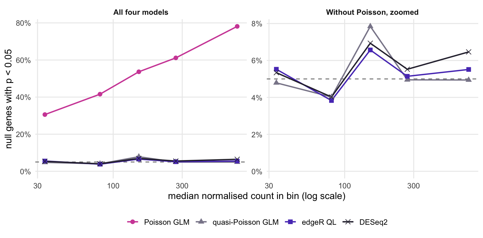
Figure 1: Share of null genes with p < 0.05, by expression. Each point is one fifth of the genes, placed at its median normalised count. The dashed line is the 5% that a valid test should give. The right panel leaves out the Poisson model and zooms in on the other three.
The damage grows with expression, as the variance ratio predicts. Among the fifth of genes with the lowest counts (median normalised count 34) the Poisson test already gives p < 0.05 for 30.6% of null genes; in the top fifth (median 720) it reaches 78.1%. Dropping weakly expressed genes therefore does nothing to rescue a Poisson analysis: the genes that remain are the ones where the assumption is furthest off. The other three models stay near the dashed line in every bin.
Diagnostic 1: the mean-variance plot
Variance larger than the mean is called overdispersion, and it is what both diagnostics below measure.
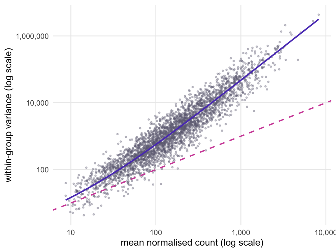
You cannot see the truth in real data, but you can see the variance. The first check needs no model. For each gene, scale the counts to a common sequencing depth, compute the mean across samples and the variance within each condition, and plot one against the other on log scales. The variance is taken within conditions and averaged, so that a real treatment effect does not inflate it.
Under a Poisson model the points would scatter around the diagonal where variance equals mean. Here the median ratio of variance to mean is 7.9, and the cloud pulls away from the diagonal as the mean rises. The violet curve is the negative binomial variance with a single dispersion for all genes, = 0.047, taken as the median over genes of (variance minus mean) divided by the squared mean. It follows the cloud; the diagonal does not.
Figure 2: Mean against within-group variance for every gene, both on log scales. The magenta dashed line is what a Poisson model assumes (variance equal to the mean); the violet curve is a negative binomial variance with one dispersion for all genes.
Diagnostic 2: the Pearson dispersion statistic
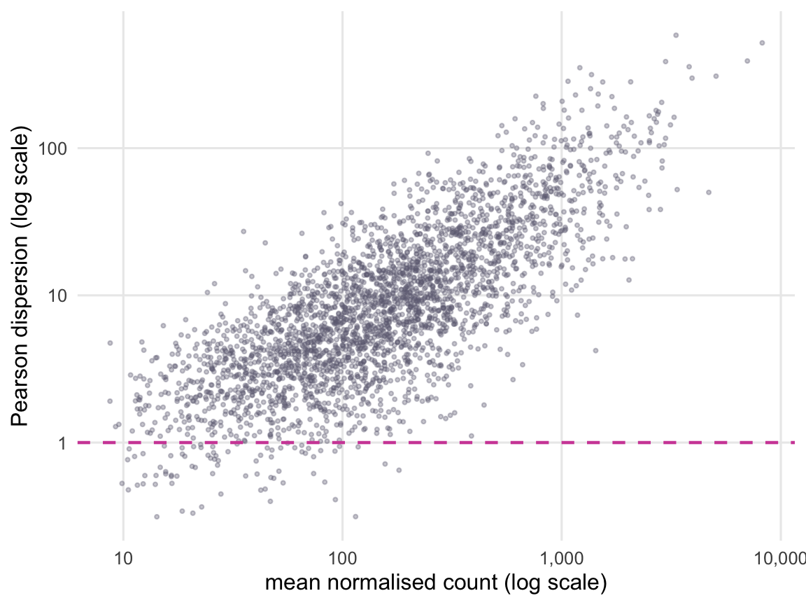
The second check uses the Poisson fit itself. For each gene, sum the squared Pearson residuals, (observed minus fitted) squared divided by fitted, over the samples, and divide the sum by the residual degrees of freedom: 8 samples minus 2 fitted means leaves 6. This is the Pearson dispersion statistic. If the Poisson model were right, it would scatter around 1, and the sum would follow a chi-square distribution on 6 degrees of freedom.
Here the median statistic is 7.7, and 88.1% of genes fail the chi-square goodness-of-fit test at the 5% level, where about 5% would fail under a Poisson model. The statistic estimates the variance ratio , so it also rises with the mean: its median is 2.7 in the lowest fifth of genes and 33.8 in the highest.
You do not need the closed-form helper to get this number for a single gene. It is what summary() of a glm() fit with family = quasipoisson prints as the dispersion parameter: base R’s summary.glm() estimates it as the sum of squared Pearson residuals divided by the residual degrees of freedom.
Figure 3: The Pearson dispersion statistic from the Poisson fit of each gene, against its mean count. A Poisson model expects values scattered around 1 (dashed line).
Quasi-Poisson: right error rate, wrong power
The quasi-Poisson model is the usual textbook answer to overdispersion when the software at hand only offers a Poisson model. It keeps the Poisson mean but lets the variance be a multiple of it, , with estimated for each gene by the Pearson statistic above. Tests divide by and compare against an F distribution; in R this is glm(family = quasipoisson) followed by anova(fit, test = "F"), which is what pois_tests() reproduces.
In the table, quasi-Poisson gets the error rate right: 5.3% of null genes below 0.05 and 2.0% false among its calls. But it calls only 98 genes and finds 32.1% of the changed ones, against 69.9% for edgeR.
The cost comes from estimating one gene at a time. With 6 residual degrees of freedom, the estimate is noisy, and the F test pays for that noise with a higher bar. The 5% cut-off for the test statistic is 3.84 when the variance is known and 5.99 on an F distribution with 6 denominator degrees of freedom. edgeR’s quasi-likelihood pipeline also estimates a quasi-dispersion for every gene, on top of the negative binomial variance, but it squeezes those estimates towards a trend fitted across all genes. That empirical Bayes step is worth 11.8 extra degrees of freedom here (prior degrees of freedom: the information borrowed from the other genes, counted as if it were extra replicates), and the cut-off drops to roughly 4.42.
To check that this is the reason, the next chunk applies the same kind of squeezing to the quasi-Poisson dispersions with limma’s squeezeVar(), using the log of the mean count as the trend covariate, and repeats the F test with the pooled degrees of freedom.
With the shared dispersion, quasi-Poisson gains 13.4 prior degrees of freedom, keeps 5.7% of null genes below 0.05, and finds 70.6% of the changed genes, close to edgeR. So the quasi-Poisson model is not badly calibrated; it is wasteful, because it treats each gene as if the other few thousand had nothing to say about its variance. It also assumes that the variance is proportional to the mean within a gene, which is off when the two conditions differ a lot in expression; in this simulation that mattered much less than the degrees of freedom.
One data set can flatter or punish the quasi-Poisson test, because with so few calls the Benjamini-Hochberg cut-off moves a lot. The next chunk repeats the whole simulation 10 more times with new seeds and keeps only the share of changed genes found.
Across those runs, quasi-Poisson found 6.1% to 25.1% of the changed genes (mean 18.6%), edgeR 64.4% to 71.6% (mean 69.1%), and quasi-Poisson with the shared dispersion 64.4% to 73.1%. So the data set above is on the kind side for quasi-Poisson: on average it finds 27% of what edgeR finds, and at best 37% of it.
What to do in practice
For RNA-seq counts with biological replicates, use a negative binomial model that shares dispersion information across genes. That is what edgeR and DESeq2 are for, and in their standard workflows they need no tuning for this. The edgeR quasi-likelihood version used above:
legacy = FALSE switches on the newer quasi-dispersion method introduced in edgeR 4.0. It estimates one common negative binomial dispersion itself, from the most highly expressed genes, so no separate estimateDisp() call is needed. The default in edgeR 4.0 is still legacy = TRUE, which stops with an error unless estimateDisp() has been run first; writing legacy = FALSE out gives the same method whichever edgeR version you run.
If you have inherited a per-gene Poisson analysis, from a general statistics package or a loop of glm() calls, run the Pearson check before trusting any of it. The helper pois_tests() has to be copied from the setup chunk, and its closed form handles one grouping factor only:
    Min.  1st Qu.   Median     Mean  3rd Qu.     Max.
  0.3133   3.5317   7.7152  18.1498  17.8413 584.7593
For any other design, fit one gene at a time and read the same number from glm(), where k is the gene’s counts and lib the normalised library sizes:
summary(glm(k ~ group +offset(log(lib)), family = quasipoisson))$dispersion
Values scattered around 1 across the whole range of expression would mean the Poisson model is adequate, as it is for technical replicates of one library. Values well above 1 that rise with the mean, as here, mean the Poisson p-values are too small, and a gene list built on them will contain many false calls, as in the table above. If a general GLM tool is all you have, quasi-Poisson is the minimum repair: it controls the error rate, but with a handful of replicates it throws away much of the power that a shared dispersion estimate would give you.
References
Marioni JC, Mason CE, Mane SM et al. 2008 Genome Research 18(9):1509-1517 (doi:10.1101/gr.079558.108)