Why CPM makes unchanged genes look down when a few genes take a big share of reads, and how TMM and DESeq2 median-of-ratios fix composition bias in RNA-seq.
Author
Pseudocount
Published
4 September 2026
You have a table of RNA-seq counts. You divide each sample by its total number of reads, multiply by a million, and compare conditions. That is counts per million (CPM), the first normalisation most people meet, and the question that follows is usually some version of “CPM or TMM, and does it matter?”
It matters when a few genes take a larger share of the reads in one condition. CPM corrects for how deeply each sample was sequenced, but not for what the reads were spent on. If a handful of highly expressed genes go up, every other gene gets a smaller slice of the same library, and CPM reports that smaller slice as down-regulation. In the simulation below, 20 of 4,000 genes go up 10-fold. Under plain CPM the typical unchanged gene shows a log2 fold change of -0.55, and an edgeR test on raw library sizes calls 1,457 of 3,972 tested unchanged genes significant at 5% FDR. With TMM normalisation the median shift is -0.001 and the false calls drop to 0.
Setup: packages and helper functions
suppressPackageStartupMessages({library(edgeR)library(DESeq2)library(ggplot2)})stopifnot(packageVersion("edgeR") >="4.0.0", # glmQLFit(legacy = FALSE) needs 4.0.0packageVersion("DESeq2") >="1.40",packageVersion("ggplot2") >="3.4.0")fmt <-function(x, d =2) formatC(x, format ="f", digits = d)fmtn <-function(x) formatC(x, format ="d", big.mark =",")pct <-function(x, d =1) formatC(100* x, format ="f", digits = d)violet <-"#5a3fc0"; magenta <-"#d14fa6"; grey <-"#8a8797"; grey_dark <-"#3d3b4a"theme_set(theme_minimal(base_size =12) +theme(panel.grid.minor =element_blank(),plot.background =element_rect(fill ="white", colour ="white")))
Why dividing by the total goes wrong
Sequencing does not count molecules; it samples a fixed number of reads from the pool of cDNA. What you observe for each gene is its share of that pool. If the up genes held a fraction of the reads in condition A and rise -fold in condition B, the reads left for everything else fall from to of the library. A gene whose absolute expression did not change therefore shows, after dividing by the total, a log2 fold change of
Nothing about the replicates or the test enters this expression. The shift is a property of the normalisation, and more replicates only make it more significant.
The setup
The simulation has 4,000 genes and 3 samples per condition. Counts are negative binomial with dispersion 0.05, which is a biological coefficient of variation of about 22%, and library sizes are drawn between 8 and 12 million reads. The 20 genes that change together take 5% of the reads in condition A; in condition B they go up 10-fold and their share rises to 34%. The other 3,980 genes keep exactly the same expression, so their true log2 fold change is zero. The formula above predicts that total-count scaling will put them at -0.54.
n_per_group <-3# replicates per conditionphi <-0.05# negative binomial dispersion (biological CV about 22%)lib_range <-c(8e6, 12e6)n_rep <-3# simulated datasets per setting in the fold-change sweepn_rep_frac <-10# and in the fraction sweep, whose ratios are noisierfc_frac <-3# fold change used in the last sweepsimulate_counts <-function(G =4000, up =1:20, share =NULL, fc =10,n = n_per_group, disp = phi) { w <-rlnorm(G, meanlog =0, sdlog =1.5) # baseline expression shapeif (!is.null(share)) { # fix the up genes' share of reads in A w[-up] <- w[-up] /sum(w[-up]) * (1- share) w[up] <- share /length(up) } else { w <- w /sum(w) } pA <- w pB <- w; pB[up] <- pB[up] * fc; pB <- pB /sum(pB) # same molecules, new proportions lib <-round(runif(2* n, lib_range[1], lib_range[2])) # sequencing depth mu <-sweep(cbind(matrix(pA, G, n), matrix(pB, G, n)), 2, lib, "*") y <-matrix(rnbinom(length(mu), mu = mu, size =1/ disp), nrow = G)storage.mode(y) <-"integer"dimnames(y) <-list(paste0("gene", seq_len(G)),paste0(rep(c("A", "B"), each = n), seq_len(2* n)))list(y = y, group =factor(rep(c("A", "B"), each = n)),changed =seq_len(G) %in% up,shareB =sum(pB[up]),expected =log2(sum(pB[-up]) /sum(pA[-up]))) # what total-count scaling will show}share_A <-0.05; fc_true <-10set.seed(404)sim <-simulate_counts(share = share_A, fc = fc_true)y <- sim$y; group <- sim$groupn_genes <-nrow(y)n_changed <-sum(sim$changed)n_unchanged <- n_genes - n_changedshare_B <- sim$shareBexpected_offset <- sim$expectedexpected_ratio <-2^expected_offsetbcv <-sqrt(phi)
Two assumptions carry the result. The first is that only a small minority of genes change, which is what TMM and median-of-ratios rely on; the last section breaks it on purpose. The second is that the changed genes are highly expressed, because a gene has to hold a real share of the library to move everyone else: in the formula, a small keeps the shift small even for a large .
Three ways to scale the same counts
Below, each gene’s log2 fold change is computed three ways: dividing by the raw library size (plain CPM), by the TMM effective library size from edgeR, and by the DESeq2 median-of-ratios size factor.
lib_raw <-colSums(y)d <-DGEList(y, group = group)d_tmm <-normLibSizes(d) # TMM is the default methodeff_lib <- lib_raw * d_tmm$samples$norm.factors # effective library sizessf_mor <-estimateSizeFactorsForMatrix(y) # DESeq2 median-of-ratioslog2_ratio <-function(scale) { z <-sweep(y, 2, scale, "/")log2(rowMeans(z[, group =="B"]) /rowMeans(z[, group =="A"]))}expressed <-rowMeans(y) >=10unchanged <-!sim$changed & expressedma <-data.frame(A =log2(rowMeans(sweep(y, 2, lib_raw /1e6, "/")) +0.5),lfc_cpm =log2_ratio(lib_raw),lfc_tmm =log2_ratio(eff_lib),lfc_mor =log2_ratio(sf_mor),changed = sim$changed)[expressed, ]med_cpm <-median(ma$lfc_cpm[!ma$changed])med_tmm <-median(ma$lfc_tmm[!ma$changed])med_mor <-median(ma$lfc_mor[!ma$changed])n_unch_expr <-sum(unchanged)tmm_ratio <-exp(mean(log(d_tmm$samples$norm.factors[group =="B"]))) /exp(mean(log(d_tmm$samples$norm.factors[group =="A"])))cpm_drop <-1-2^med_cpm # apparent fractional drop of a typical unchanged gene
TMM, the trimmed mean of M-values (Robinson and Oshlack 2010), compares each sample with a reference sample gene by gene. For every gene it takes the log ratio between the two (the M-value) and the average log expression (the A-value), trims 30% of the M-values from each tail and 5% of the A-values from each tail, and takes a weighted mean of what is left. The 20 up genes have extreme M-values, so they are trimmed away and the factor is set by the genes that did not change. In edgeR the result is stored as a normalisation factor that multiplies the library size into an effective library size.
Median-of-ratios, the method from Anders and Huber (2010) that DESeq2 uses (Love et al. 2014), builds a pseudo-reference sample from the geometric mean of each gene across all samples, then takes the median over genes of each sample’s ratio to that reference. Genes with a zero in any sample are left out. A median barely moves when 20 genes out of thousands shift, so the size factor again reflects the unchanged majority.
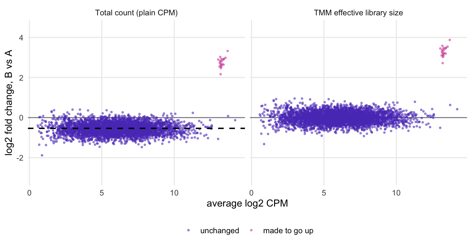
Figure 1: MA plots of the same simulated counts, scaled by total count (left) and by TMM effective library size (right). Violet: unchanged genes; magenta: the genes that were made to go up. The dashed line is the shift that total-count scaling must produce.
The left panel is what plain CPM does. The violet cloud of unchanged genes does not sit on zero: it sits on the dashed line, with a median log2 fold change of -0.55 against the predicted -0.54. On the original scale a typical unchanged gene looks 32% lower in condition B. In the right panel TMM has put the cloud back on zero: the median is -0.001, and median-of-ratios gives -0.004.
TMM gets there by giving the condition B samples smaller effective library sizes. The ratio of normalisation factors, B over A, is 0.68; the ratio needed to cancel the shift exactly is 0.69. In plain words, TMM has worked out that part of each B library was spent on the 20 up genes, and it stops counting those reads when it scales everything else.
What the shift does to a differential expression test
A shift of half a log2 unit is not a cosmetic problem once a test sees it. Here the same counts go through the edgeR quasi-likelihood pipeline (filterByExpr, estimateDisp, glmQLFit, glmQLFTest, with legacy = FALSE set explicitly so that older and newer edgeR versions fit the same model) and the standard DESeq2 pipeline, each run twice: once with only total-count scaling, once with its own composition-aware normalisation. For edgeR, total-count scaling is normLibSizes(method = "none"), which is what you get if you skip the normalisation step; for DESeq2 it means setting the size factors to the library sizes before calling DESeq().
Neither package does this by default. The edgeR help page for normLibSizes() makes the same point with a toy example (CPM on raw library sizes makes two samples look different, normalised library sizes make most of their CPMs equal), and the DESeq2 vignette lists size factor estimation (estimateSizeFactors(), median-of-ratios by default) as the first step inside DESeq(). The DESeq2 total-count arm below needed a deliberate override; in real work DESeq2 users meet this bias through hand-set size factors or by starting from CPM or TPM tables.
With total-count scaling, 52% of the unchanged genes have in edgeR and 53% in DESeq2, where 5% is what a calibrated test gives. At a false discovery rate of 5%, edgeR calls 1,457 of 3,972 tested unchanged genes and DESeq2 calls 1,526 of 3,980. All 1,457 of the edgeR false calls are down-regulated: this is the shift from the MA plot turned into a gene list.
With the recommended normalisation the pile disappears. edgeR with TMM makes 0 false calls and 4.7% of unchanged genes fall below . DESeq2 with median-of-ratios makes 5 (4 up, 1 down), with 5.2% below . That is still a false discovery proportion of 20% among its calls, well above the 5% target, but it is a different problem: with only 20 real changes, a handful of false calls is a large proportion, and DESeq2 runs slightly liberal with 3 replicates per group. A control run on data where nothing changes at all shows this directly:
set.seed(405)sim0 <-simulate_counts(share = share_A, fc =1) # the same genes, no changenull_edger <-run_edger(sim0$y, sim0$group, "TMM")null_deseq2 <-run_deseq2(sim0$y, sim0$group, FALSE)p05_null_edger <-mean(null_edger$p <0.05, na.rm =TRUE)p05_null_deseq2 <-mean(null_deseq2$p <0.05, na.rm =TRUE)
With no change anywhere there is no composition effect to correct, yet DESeq2 still puts 5.9% of genes below , against 5.3% for edgeR. The excess comes from the test with 3 replicates, not from the scaling. Every analysis in the table finds 20 of the 20 genes that really changed, so skipping composition-aware normalisation buys no power. It only adds false positives.
The median column in the table is the fitted log fold change from each test, so it differs a little from the direct ratios of scaled counts in the MA plot; both put the unchanged genes at zero once the scaling accounts for composition.
One DESeq2 detail, since the threshold here is 5%: the alpha argument of results() defaults to 0.1, and that value sets the target for its independent filtering. If you report genes at FDR 5%, pass alpha = 0.05 as done above.
How large the shift gets
The size of the bias depends on how much of the library the changing genes capture. The next simulation keeps the 20 genes at 5% of the reads in condition A and varies how far they go up, with 3 simulated datasets per setting.
fold_long <-rbind(data.frame(fc = sweep_fold$fc, value = sweep_fold$total, scaling ="total count (CPM)"),data.frame(fc = sweep_fold$fc, value = sweep_fold$TMM, scaling ="TMM"),data.frame(fc = sweep_fold$fc, value = sweep_fold$MoR, scaling ="median-of-ratios"))fold_long$scaling <-factor(fold_long$scaling, levels =unique(fold_long$scaling))ggplot(fold_long, aes(fc, value, colour = scaling, shape = scaling)) +geom_hline(yintercept =0, colour = grey) +geom_line(data = sweep_fold, aes(fc, expected), inherit.aes =FALSE,linetype ="dashed", colour ="black") +geom_line(aes(linetype = scaling)) +geom_point(size =2.4) +scale_x_continuous(trans ="log2", breaks = fold_grid) +scale_colour_manual(values =c(magenta, violet, grey_dark), name =NULL) +scale_shape_manual(values =c(16, 17, 15), name =NULL) +scale_linetype_manual(values =c("solid", "solid", "dotted"), name =NULL) +labs(x =paste0("fold change of the ", n_changed, " up genes (log scale)"),y ="median log2FC of unchanged genes") +theme(legend.position ="bottom")
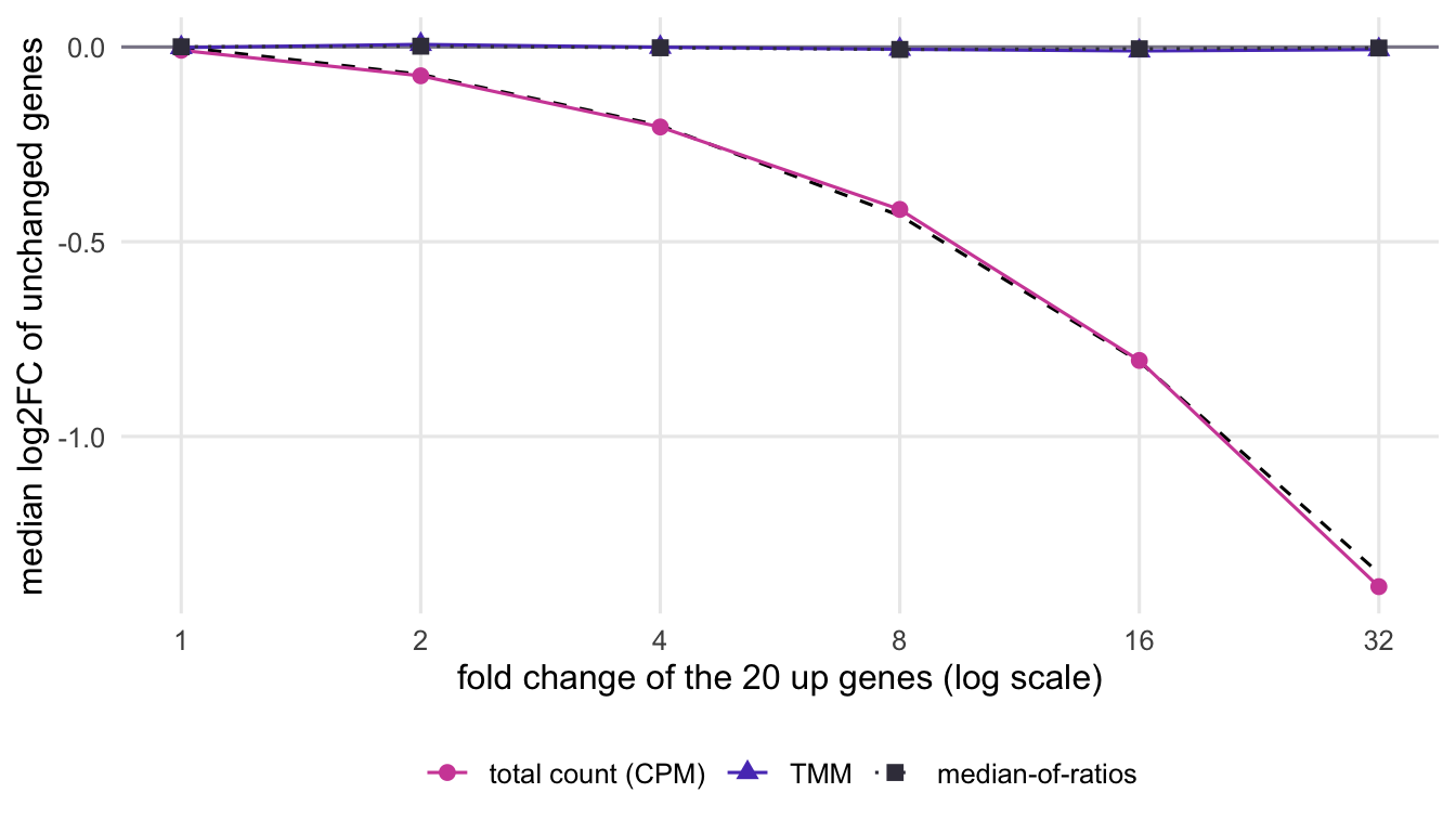
Figure 2: Median log2 fold change of the unchanged genes as a handful of highly expressed genes are pushed further up. Total-count scaling follows the expected shift (dashed line); TMM and median-of-ratios stay near zero, where their lines lie on top of each other.
At a 2-fold change the unchanged genes shift by only -0.07 under total-count scaling, small next to the gene-to-gene scatter in the MA plot. At 32-fold, where the up genes take 63% of the reads in condition B, the shift is -1.39, which is a 2.6-fold apparent drop for every other gene. Across the whole range TMM and median-of-ratios stay within 0.02 of zero.
Where TMM and median-of-ratios stop working
Both methods assume that most genes do not change, or that the changes up and down roughly balance. That assumption is the price of estimating the scaling from the genes themselves. To see what happens when it fails, the last simulation picks a growing fraction of genes at random and makes them all go up 3-fold, with no genes going down, averaging over 10 simulated datasets per setting.
frac_long <-rbind(data.frame(frac = sweep_frac$frac, value = sweep_frac$total, scaling ="total count (CPM)"),data.frame(frac = sweep_frac$frac, value = sweep_frac$TMM, scaling ="TMM"),data.frame(frac = sweep_frac$frac, value = sweep_frac$MoR, scaling ="median-of-ratios"))frac_long$scaling <-factor(frac_long$scaling, levels =unique(frac_long$scaling))ggplot(frac_long, aes(100* frac, value, colour = scaling, shape = scaling)) +geom_hline(yintercept =0, colour = grey) +geom_line(aes(linetype = scaling)) +geom_point(size =2.4) +scale_colour_manual(values =c(magenta, violet, grey_dark), name =NULL) +scale_shape_manual(values =c(16, 17, 15), name =NULL) +scale_linetype_manual(values =c("solid", "solid", "dotted"), name =NULL) +labs(x =paste0("genes that go up ", fc_frac, "-fold (%)"),y ="median log2FC of unchanged genes") +theme(legend.position ="bottom")
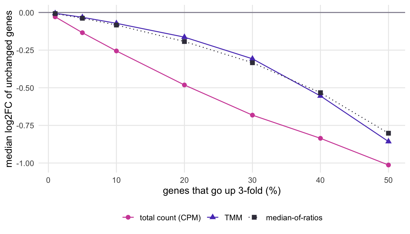
Figure 3: The same measurement when a growing fraction of randomly chosen genes goes up, all in the same direction. Both composition-aware methods drift as the changed genes approach half of all genes.
With 5% of genes up, TMM leaves a shift of -0.03 against -0.13 for total-count scaling, removing 76% of the bias. With 20% of genes up it leaves -0.16 (median-of-ratios -0.19) against -0.48, which still removes most of it (66%). When half the genes go up, TMM is at -0.86 and median-of-ratios at -0.80, not far from the -1.01 of plain CPM: only 15% of the bias is removed. There is no majority of unchanged genes left to anchor on, and no method that uses only the sample’s own genes can tell “half the genes went up” from “the other half went down”.
Why does TMM already leave a shift at 5%, when it trims 30% from each tail? A 3-fold change is not extreme next to the noise of low-count genes, so many of the randomly chosen genes stay inside the untrimmed middle, and because they all move the same way they pull the trimmed mean and the median with them. The 20 genes of the first example escaped this because they were highly expressed and changed 10-fold.
A one-sided global change like this can happen, for example, when a treatment raises transcription across most of the genome. The reference then has to come from outside the genes being compared, usually spike-in RNA added in a fixed amount per cell. Spike-ins added per microgram of total RNA, a common way of using them, do not help here, because the total RNA is exactly what changed. DESeq2 can compute size factors from such a control set with the controlGenes argument of estimateSizeFactors(), and its vignette describes this case.
What to do in practice
If you use edgeR, run normLibSizes() before anything that uses library sizes, and take CPM values from cpm() on the normalised object rather than from your own division by column sums:
library(edgeR)d <-DGEList(counts, group = group)keep <-filterByExpr(d)d <- d[keep, , keep.lib.sizes =FALSE]d <-normLibSizes(d) # TMM by default; calcNormFactors(d) in older codelogcpm <-cpm(d, log =TRUE) # uses the TMM effective library sizes
normLibSizes() is the newer name for calcNormFactors(). Both exist in the edgeR version used here (4.8.2), the edgeR documentation says the two are equivalent and that calcNormFactors() will eventually be retired, and normLibSizes() first appeared in edgeR 3.42.0. The version guard at the top asks for edgeR 4.0.0 because of the legacy argument of glmQLFit(). The default method of normLibSizes() is TMM. The cpm() method for a DGEList has normalized.lib.sizes = TRUE by default, so after normLibSizes() it returns TMM-normalised CPM. cpm(log = TRUE) also adds a prior count before taking the log, which changes low-count genes in its own way; that is covered in an earlier post.
If you use DESeq2, the standard DESeq() call already estimates median-of-ratios size factors. For normalised values outside the test:
Two habits catch the problem in real data. First, do not run a differential expression test on a table of CPM or TPM values exported from another tool: both are shares of each sample’s total and carry the same composition bias, and they have also lost the count information the tests need. Second, look at an MA plot after normalisation. If the dense cloud of genes is not centred on zero, either the normalisation was skipped or the assumption that most genes are unchanged does not hold for your experiment, and those two need different fixes. The reverse does not follow: TMM and median-of-ratios centre the bulk of genes by construction, so a centred plot cannot rule out a global shift. Only an external reference such as spike-ins can.