Paired samples in DESeq2: what ignoring patient costs
experimental design
DESeq2
edgeR
limma
RNA-seq
Paired design in DESeq2, edgeR and limma: what dropping patient from the design costs in power, whether it inflates FDR, and how to fix the not full rank error.
You have tumour and normal tissue from the same patients, or blood taken before and after treatment from the same volunteers. Does patient belong in the design formula, and what happens if you leave it out? When every patient gives one sample per condition and patients differ, leaving it out does not inflate false positives. It throws away power, and when patients differ a lot, nearly all of it. In the simulation below, with 4 patients and a moderate patient effect, the paired analysis ~ patient + condition finds between 68% and 69% of the truly changed genes in DESeq2, edgeR and limma-voom. The unpaired analysis ~ condition finds 23% in DESeq2 and next to nothing in edgeR and limma-voom, which called no gene at all in every one of their 20 analyses at this setting, and its realised false discovery rate does not rise. When patients do not differ at all, the patient term costs little: on average 4.6% of the changed genes in DESeq2 with 4 patients, and less in the other cases.
A paired design (also called a blocked design) is one where each biological unit, here a patient, gives a sample in every condition. The pairing is part of the experiment, so it has to be part of the model.
Why the pairing matters
Take one gene and write and for its log expression in patient before and after treatment. Each patient has their own baseline : some people express the gene at a much higher level than others, for reasons that have nothing to do with the treatment. In a design where every patient gives one sample per condition, the estimated treatment effect is the average of the within-patient differences,
and appears in both terms of each difference, so it cancels. This is true whether or not the model knows about patients. What changes is the noise estimate. With ~ patient + condition, the residual variance is the variation within a patient. With ~ condition, the model has nowhere to put , so the patient-to-patient spread is added to the residual variance. The test then divides a clean estimate by an inflated standard error. The statistic shrinks, the p-values move towards 1, and both power and the false positive rate go down.
The setup
Each simulated experiment has patients, each giving one control and one treated sample, for 3,000 genes. The counts are negative binomial, the usual model for RNA-seq read counts. The first 300 genes change with treatment, by a log2 fold change of plus or minus 1; the rest do not change. Every gene also gets a patient effect: for each patient, a log2 shift drawn from a normal distribution with standard deviation , the same shift in that patient’s control and treated sample.
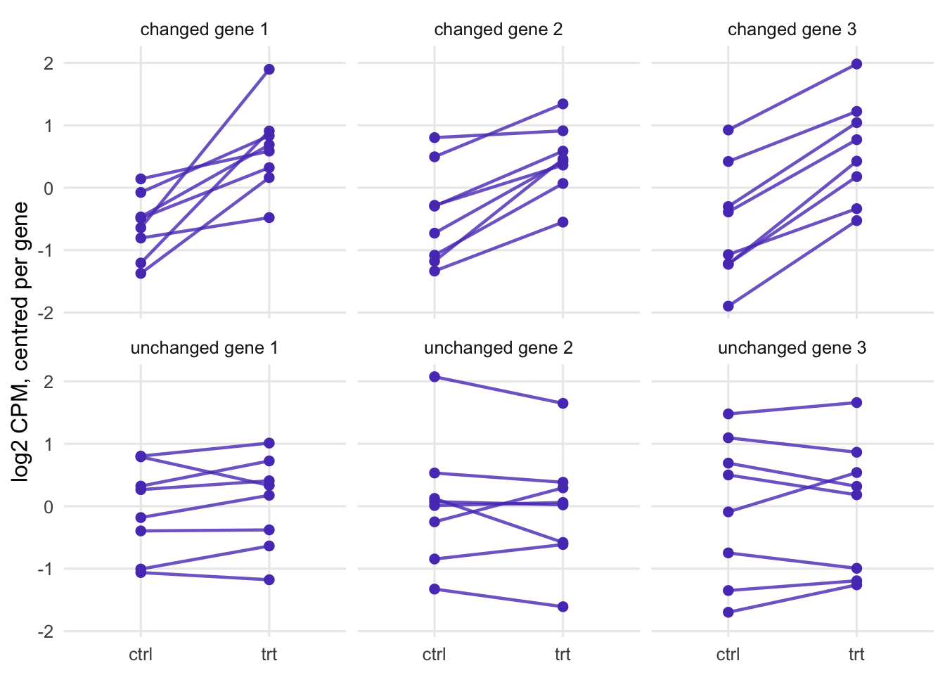
How large is a patient effect with = 0.4? A useful yardstick is the share of a gene’s sample-to-sample variance (on the log scale) that comes from patients. For a gene with a mean count of 150 and the dispersion used here, that share is 23% at = 0.2, 55% at 0.4 and 83% at 0.8. The figure shows the largest setting with 8 patients. Each patient’s two samples are joined by a line: the lines start far apart, and in the changed genes they climb by a similar amount.
Figure 1: One simulated experiment with the larger number of patients and the largest patient effect: log2 counts per million, centred on each gene’s mean, for three changed genes (top) and three unchanged genes (bottom). Each line joins the control and treated sample of one patient.
The assumptions that carry the argument: the patient effect adds to the treatment effect on the log scale (every patient responds by the same fold change, apart from noise), and it is independent between genes. The first one matters most. If patients respond differently to the treatment, that variation is noise for the average treatment effect in both models, and pairing cannot remove it.
Each experiment is analysed six ways: DESeq2, edgeR and limma-voom, each with ~ condition and with ~ patient + condition. DESeq2 (Love et al. 2014) runs its standard workflow, with alpha = 0.05 in results() because genes are called at a 5% FDR (its help page asks for alpha to match the cut-off when it is not 0.1). edgeR runs the quasi-likelihood pipeline (Chen et al. 2016): filterByExpr(), normLibSizes(), then glmQLFit() with robust = TRUE and legacy = FALSE (the new method, which is the default from edgeR 4.2), and glmQLFTest(). limma-voom (Law et al. 2014) runs voom(), lmFit() and eBayes() on the same filtered and normalised data. The filter uses group = condition, so both models test the same genes. The simulator and the three analyses live in a small file that the page runs:
# Simulator and the three analyses used in the post (sourced by paired_sim.R)G <-3000# genes per simulated experimentn_de <-300# the first n_de genes change with treatmenttrue_lfc <-1# log2 fold change of the changed genes (up or down)sd_grid <-c(0, 0.2, 0.4, 0.8) # SD of the log2 patient effectn_grid <-c(4, 8) # patients, each with one ctrl and one trt samplemake_samples <-function(n) data.frame(patient =factor(paste0("P", rep(seq_len(n), 2))),condition =factor(rep(c("ctrl", "trt"), each = n)))sim_data <-function(n, sd_p) { mu0 <-exp(rnorm(G, log(150), 1.3)) # baseline mean count phi <- (0.05+1/ mu0) *exp(rnorm(G, 0, 0.3)) # NB dispersion within a patient lfc <-c(sample(c(-1, 1) * true_lfc, n_de, TRUE), rep(0, G - n_de)) samples <-make_samples(n) u <-matrix(rnorm(G * n, 0, sd_p), G, n) # log2 patient effect, per gene lf <-outer(lfc, samples$condition =="trt") + u[, as.integer(samples$patient)] mu <- mu0 *2^lf *rep(runif(2* n, 0.8, 1.25), each = G) counts <-matrix(rnbinom(G *2* n, mu = mu, size =1/ phi), G, 2* n)storage.mode(counts) <-"integer"list(counts = counts, samples = samples, lfc = lfc)}is_de <-seq_len(G) <= n_derun_deseq2 <-function(d, design) { dds <-DESeqDataSetFromMatrix(d$counts, d$samples, design) dds <-DESeq(dds, quiet =TRUE) res <-results(dds, name ="condition_trt_vs_ctrl", alpha =0.05)list(p = res$pvalue, padj = res$padj)}run_edger_limma <-function(d, design) { X <-model.matrix(design, d$samples) y <-DGEList(d$counts) keep <-filterByExpr(y, group = d$samples$condition) # same genes for both designs y <-normLibSizes(y[keep, , keep.lib.sizes =FALSE]) fit_ql <-glmQLFit(y, X, robust =TRUE, legacy =FALSE) p_edger <-glmQLFTest(fit_ql, coef ="conditiontrt")$table$PValue p_limma <-eBayes(lmFit(voom(y, X), X))$p.value[, "conditiontrt"] out <-function(p) { full <-rep(NA_real_, G); full[keep] <- p adj <-rep(NA_real_, G); adj[keep] <-p.adjust(p, "BH")list(p = full, padj = adj) }list(edgeR =out(p_edger), limma =out(p_limma))}score <-function(r) { called <-!is.na(r$padj) & r$padj <0.05c(calls =sum(called), # genes called at 5% FDRpower =sum(called & is_de) / n_de, # changed genes foundfdp =if (any(called)) mean(!is_de[called]) else0, # false discovery proportionfpr =mean(r$p[!is_de] <0.05, na.rm =TRUE)) # null genes with p < 0.05}
The grid crosses 2 numbers of patients with 4 sizes of patient effect and repeats each combination 10 times. Power counts a changed gene as missed if it was filtered out. Within one repeat, the six analyses see exactly the same counts. With 10 x 8 experiments and two DESeq2 fits each, the grid takes several minutes, so it runs as a separate script that writes one row per experiment, package and model to a CSV file, which this page reads. The file records the versions that produced it: DESeq2 1.42.0, edgeR 4.0.16 and limma 3.58.1.
# The simulation grid behind the post. Run from this folder: Rscript paired_sim.R# Writes paired_sim-results.csv: one row per simulated experiment x package x model,# with the package versions that produced it.suppressPackageStartupMessages({ library(DESeq2); library(edgeR); library(limma) })stopifnot(packageVersion("DESeq2") >="1.40", packageVersion("edgeR") >="4.0.0",packageVersion("limma") >="3.58")source("paired_sim_functions.R")out_file <-if (length(commandArgs(TRUE))) commandArgs(TRUE)[1] else"paired_sim-results.csv"n_rep <-10designs <-list(unpaired =~ condition, paired =~ patient + condition)set.seed(2026)res <-list()for (r inseq_len(n_rep)) for (n in n_grid) for (sd_p in sd_grid) { d <-sim_data(n, sd_p)for (m innames(designs)) { fits <-c(list(DESeq2 =run_deseq2(d, designs[[m]])), run_edger_limma(d, designs[[m]]))for (k innames(fits)) res[[length(res) +1]] <-data.frame(rep = r, n = n, sd_p = sd_p, method = k,model = m, t(score(fits[[k]]))) }}res <-do.call(rbind, res)res$DESeq2_version <-as.character(packageVersion("DESeq2"))res$edgeR_version <-as.character(packageVersion("edgeR"))res$limma_version <-as.character(packageVersion("limma"))write.csv(res, out_file, row.names =FALSE)
res <-read.csv("paired_sim-results.csv")n_rep <-max(res$rep)agg <-aggregate(cbind(calls, power, fdp, fpr) ~ method + model + n + sd_p, res, mean)agg$power_max <-aggregate(power ~ method + model + n + sd_p, res, max)$poweragg$no_calls <-aggregate(calls ~ method + model + n + sd_p, res, function(x) sum(x ==0))$calls# realised FDR among the experiments that called anythingfdr_called <-aggregate(fdp ~ method + model + n + sd_p, res[res$calls >0, ], mean)agg <-merge(agg, setNames(fdr_called, c("method", "model", "n", "sd_p", "fdr_called")),all.x =TRUE, sort =FALSE)
meths <-c("DESeq2", "edgeR", "limma")a <-function(meth, mod, nn, s, v) agg[agg$method == meth & agg$model == mod & agg$n == nn & agg$sd_p == s, v]rng <-function(mod, nn, s, v) range(sapply(meths, a, mod = mod, nn = nn, s = s, v = v))pct_rng <-function(x) if (pct(x[1]) ==pct(x[2])) pct(x[1]) elsepaste(pct(x[1]), "to", pct(x[2]))n_head <- n_grid[1]; sd_head <- sd_grid[3]pow_pair_head <-rng("paired", n_head, sd_head, "power")pow_unp_head_deseq2 <-a("DESeq2", "unpaired", n_head, sd_head, "power")n_zero_el <-sum(res$calls[res$model =="unpaired"& res$n == n_head & res$sd_p == sd_head & res$method !="DESeq2"] ==0)zero_txt <-if (n_zero_el ==2* n_rep) "every one"else n_zero_elpow_unp_top_max <-max(res$power[res$model =="unpaired"& res$sd_p ==max(sd_grid)])z_ex <-5# an example test statistic under the paired modelpow_unp_8 <-rng("unpaired", n_grid[2], sd_head, "power")pow_pair_8 <-rng("paired", n_grid[2], sd_head, "power")# cost of the patient term when there is no patient effect (unpaired minus paired power)cost0 <-sapply(meths, function(m) sapply(n_grid, function(nn)a(m, "unpaired", nn, 0, "power") -a(m, "paired", nn, 0, "power")))dimnames(cost0) <-list(paste(n_grid, "patients"), meths)cost_other <-max(cost0[2, "DESeq2"], cost0[, c("edgeR", "limma")])cost_el <-range(cost0[, c("edgeR", "limma")])# patient share of log-scale variance for a typical gene (delta method, size factor 1)mu_typ <-150; phi_typ <-0.05+1/ mu_typv_within <- (1/ mu_typ + phi_typ) /log(2)^2share <- sd_grid^2/ (sd_grid^2+ v_within)shrink <-sqrt(1- share) # factor by which ~ condition shrinks the test statistic# residual degrees of freedom of the two modelsdf_res <-sapply(n_grid, function(nn) { s <-make_samples(nn)c(unpaired =2* nn -qr(model.matrix(~ condition, s))$rank,paired =2* nn -qr(model.matrix(~ patient + condition, s))$rank)})colnames(df_res) <-paste(n_grid, "patients")# false positives and false discoveriesbh_bound <-0.05* (1- n_de / G) # BH controls the FDR at 5% times the null sharefpr_pair_rng <-range(agg$fpr[agg$model =="paired"])fpr_unp_top <-max(agg$fpr[agg$model =="unpaired"& agg$sd_p ==max(sd_grid)])unp_big <- agg$model =="unpaired"& agg$sd_p >= sd_headfdr_unp_big <-max(agg$fdr_called[unp_big], na.rm =TRUE)n_nocall_cells <-sum(agg$no_calls[unp_big] == n_rep)fdr_pair <-tapply(agg$fdp[agg$model =="paired"], agg$method[agg$model =="paired"], mean)fdr_deseq2_0 <-c(unpaired =a("DESeq2", "unpaired", n_head, 0, "fdp"),paired =a("DESeq2", "paired", n_head, 0, "fdp"))round(cost0, 3); df_res
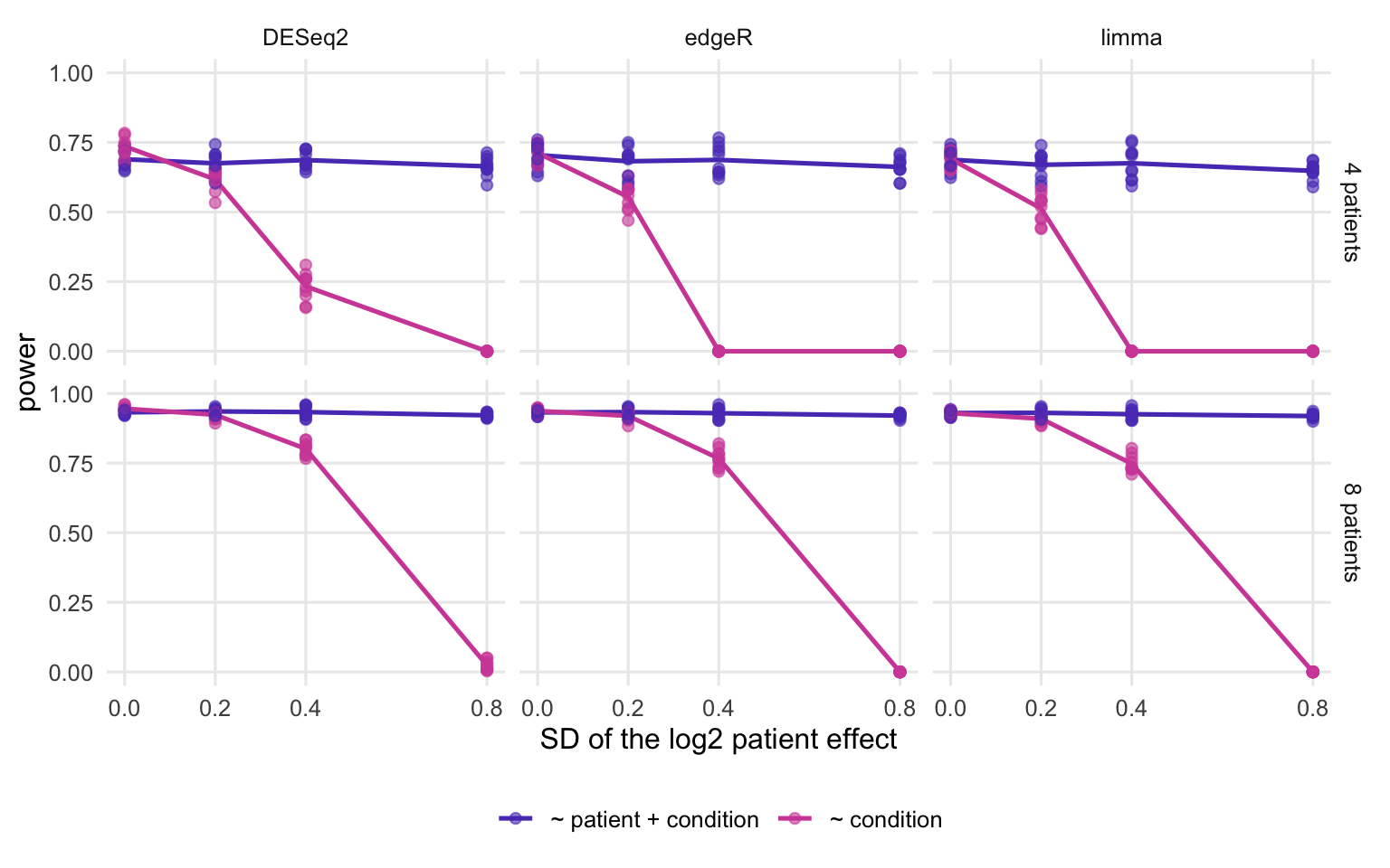
Figure 2: Power at a 5% FDR cut-off as the patient effect grows. Columns: package; rows: number of patients. Lines join the averages; dots are the single simulated experiments.
Power at a 5% FDR cut-off, averaged over 10 simulated experiments per cell. For ~ condition, the largest value in any single experiment is in brackets.
package
model
patients
SD 0
SD 0.2
SD 0.4
SD 0.8
DESeq2
~ patient + condition
4
69%
68%
69%
66%
DESeq2
~ condition
4
74% (78%)
62% (65%)
23% (31%)
0% (0%)
edgeR
~ patient + condition
4
70%
68%
69%
66%
edgeR
~ condition
4
71% (75%)
55% (63%)
0% (0%)
0% (0%)
limma
~ patient + condition
4
69%
67%
68%
65%
limma
~ condition
4
69% (72%)
51% (58%)
0% (0%)
0% (0%)
DESeq2
~ patient + condition
8
93%
94%
93%
92%
DESeq2
~ condition
8
95% (96%)
92% (94%)
80% (83%)
2% (5%)
edgeR
~ patient + condition
8
93%
93%
93%
92%
edgeR
~ condition
8
94% (95%)
92% (94%)
77% (82%)
0% (0%)
limma
~ patient + condition
8
93%
93%
93%
92%
limma
~ condition
8
93% (94%)
91% (93%)
75% (80%)
0% (0%)
The paired analysis does not care how different the patients are: within each panel its power is flat, because the patient effect cancels from every comparison it makes. The unpaired analysis matches it only when there is no patient effect. With 4 patients and = 0.4, it finds 23% of the changed genes in DESeq2 and next to nothing in the other two, against 68% to 69% with the patient term. Doubling the number of patients softens the loss at that setting (75% to 80% unpaired, 93% paired), but not at the largest patient effect, where the unpaired analysis finds almost nothing at either size (at most 5.0% in any single experiment).
The loss can be read off the argument above. On the log scale, leaving the patient out multiplies the test statistic by roughly , where is the patient share of the variance. For the typical gene that factor is 0.88, 0.67 and 0.41 for the three non-zero settings. At the largest setting a gene whose test statistic would have been 5 ends up near 2.1. This is an approximation, but it shows why no FDR cut-off brings the power back: the evidence is diluted before any cut-off is applied.
Why does DESeq2 keep some power in the unpaired fit at an SD of 0.4 when edgeR and limma keep almost none? Not because it copes better with the missing term. The evidence for the changed genes is diluted in all three, and at this setting it sits close to the point where the Benjamini-Hochberg (BH) adjustment switches from calling dozens of genes to calling none, so small differences in the tail of the p-values decide which side a package lands on. DESeq2’s Wald test compares its statistic with a standard normal distribution by default (useT = FALSE in nbinomWaldTest()), treating the moderated dispersion as known. edgeR’s quasi-likelihood F-test and limma’s moderated t-test use reference distributions with finite degrees of freedom (the residual ones plus the prior ones borrowed from other genes), whose heavier tails give larger p-values for the same evidence. Rerunning DESeq2’s test on one unpaired experiment with a t reference (useT = TRUE, which by default uses the residual degrees of freedom) shows the effect:
DESeq2, normal reference      DESeq2, t reference                 edgeR QL
                      82                        0                        0
              limma-voom
                       0
In this experiment DESeq2 calls 82 genes with the normal reference and 0 with the t reference; edgeR calls 0 and limma-voom 0. The residual degrees of freedom alone are fewer than edgeR and limma use, so the t reference overstates the difference for any single gene. The point is where the calls come from: at this setting they hinge on the tail of the reference distribution, not on how well a package handles the missing patient term. With the patient term, the three packages find about the same share of the changed genes.
False discoveries: ignoring the pairing is conservative
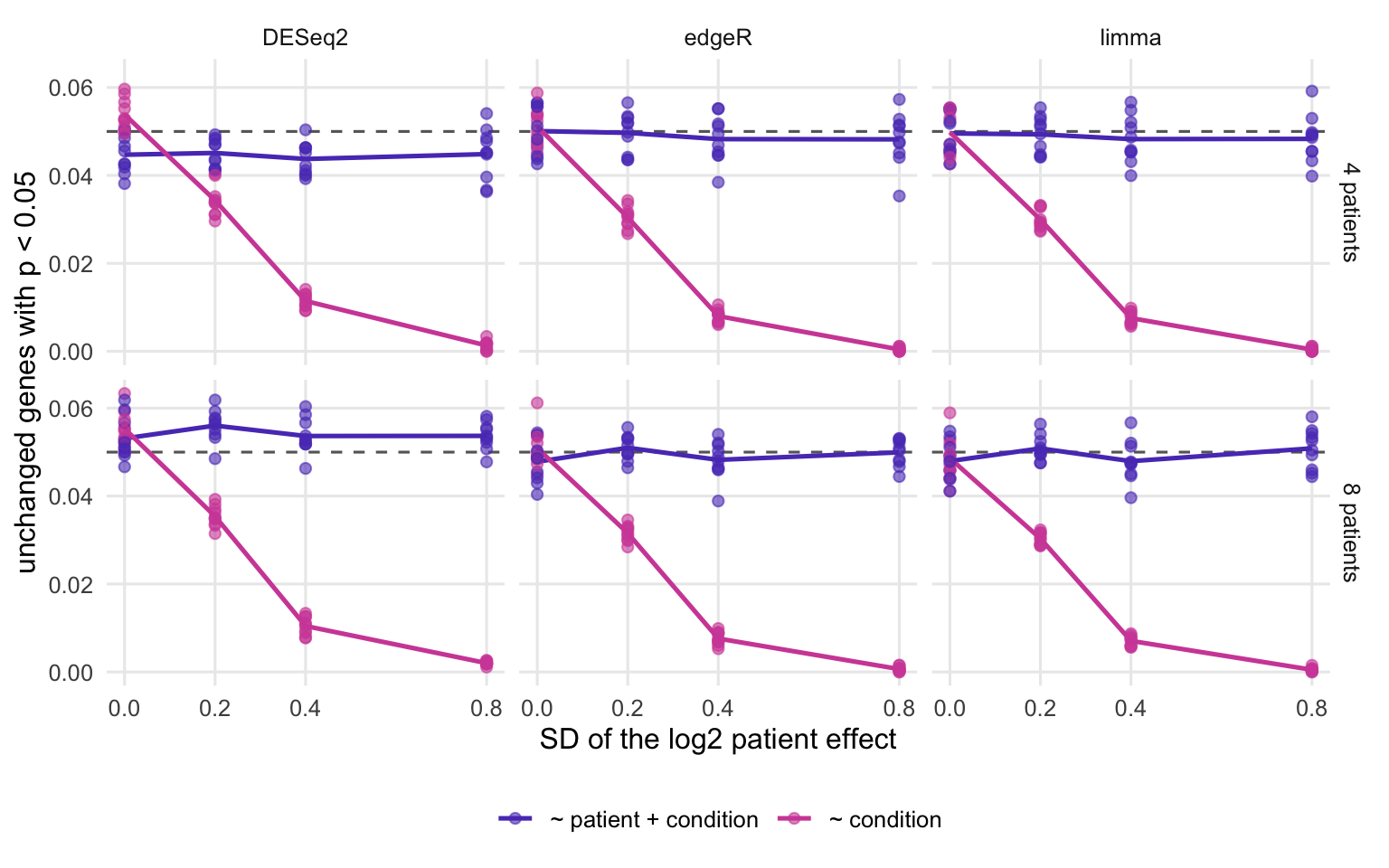
A common worry is that the wrong model produces false positives. Here it does the opposite. The next figure counts the unchanged genes with a raw p-value below 0.05, which should be 5% of them if the test is calibrated.
ggplot(agg, aes(sd_p, fpr, colour = analysis)) +geom_hline(yintercept =0.05, linetype ="dashed", colour ="grey40") +geom_line(linewidth =0.9) +geom_point(data = res, size =1.8, alpha =0.6) +facet_grid(patients ~ method) +scale_colour_manual(values =c(violet, magenta), name =NULL) +scale_x_continuous(breaks = sd_grid) +labs(x ="SD of the log2 patient effect", y ="unchanged genes with p < 0.05") + theme_pc
Figure 3: Share of unchanged genes with a raw p-value below 0.05. The dashed line marks the share expected from a calibrated test. Columns: package; rows: number of patients.
With the patient term, all three packages stay close to the line at every setting: between 4.4% and 5.6% of the unchanged genes fall below 0.05. Without it, the share falls as the patient effect grows, to at most 0.2% at the largest setting. A test that rejects a true null less often than it should is called conservative. In a p-value histogram this shows up as a ramp of null p-values towards 1, the U shape described in the post on p-value histograms.
The realised false discovery rate (the average share of false genes among those called) follows the same pattern, with one complication: an analysis that calls nothing has no false discoveries, so the table shows the number of calls next to each value and says “no calls” where none of the experiments called a gene.
Realised false discovery rate: the mean false discovery proportion over the experiments that called at least one gene at a 5% FDR cut-off, with the mean number of calls per experiment in brackets. A star marks cells where some of the 10 experiments called nothing.
package
model
patients
SD 0
SD 0.2
SD 0.4
SD 0.8
DESeq2
~ patient + condition
4
5.6% (219)
5.4% (214)
5.0% (217)
5.2% (210)
DESeq2
~ condition
4
7.1% (238)
3.3% (192)
0.1% (70)
no calls
edgeR
~ patient + condition
4
4.1% (221)
4.5% (214)
4.4% (216)
4.3% (208)
edgeR
~ condition
4
4.6% (224)
2.1% (170)
no calls
no calls
limma
~ patient + condition
4
3.8% (215)
4.2% (210)
4.1% (212)
3.8% (202)
limma
~ condition
4
4.4% (217)
1.6% (156)
no calls
no calls
DESeq2
~ patient + condition
8
6.4% (299)
7.1% (302)
6.2% (299)
6.7% (296)
DESeq2
~ condition
8
7.2% (306)
3.7% (288)
0.6% (242)
0.0% (7)
edgeR
~ patient + condition
8
4.7% (293)
5.2% (296)
4.1% (291)
4.3% (289)
edgeR
~ condition
8
5.3% (297)
2.5% (283)
0.4% (231)
no calls
limma
~ patient + condition
8
4.7% (293)
5.0% (294)
3.7% (288)
4.1% (288)
limma
~ condition
8
4.8% (293)
1.7% (278)
0.2% (225)
no calls
Without the patient term, the realised FDR falls as the patient effect grows. From an SD of 0.4 upwards, when the unpaired analysis calls anything, at most 0.6% of its calls are false on average; in 7 of those 12 cells no experiment called anything. With the patient term, the rows scatter around the target. With 90% of the genes unchanged, the BH procedure promises an FDR of at most 4.5% rather than 5%. Averaged over all 8 settings, the paired analysis has a realised FDR of 6.0% in DESeq2, 4.5% in edgeR and 4.2% in limma-voom. DESeq2 sits above that bound, and its unpaired fit does too when there is no patient effect to ignore, so this is a property of DESeq2 in this simulation rather than of the pairing; the normal reference distribution of its Wald test, discussed above, is consistent with it.
The conservative behaviour depends on the balance of the design: every patient gives one sample to each condition, so the patient effects cancel from the estimate. With incomplete pairs, or with patients who differ between conditions in some systematic way, they no longer cancel exactly, and the reassurance above does not carry over. This post does not simulate that case.
The honest cost: degrees of freedom
Adding patient is not free. Each patient adds a coefficient to the model, and each coefficient uses up a residual degree of freedom: one of the independent pieces of information left over for estimating the noise. With 4 patients, the unpaired model has 6 residual degrees of freedom and the paired model 3; with 8 patients, 14 against 7.
Halving the information about the noise sounds serious, but none of the three packages estimates a gene’s variance from that gene alone. All of them borrow strength from the other genes (empirical Bayes moderation of the dispersion or variance). limma reports the size of the borrowing directly, as a number of prior degrees of freedom added to each gene’s own. For one experiment with 4 patients and no patient effect:
set.seed(7)d0 <-sim_data(n_grid[1], 0)y0 <-DGEList(d0$counts)y0 <-normLibSizes(y0[filterByExpr(y0, group = d0$samples$condition), , keep.lib.sizes =FALSE])df_limma <-sapply(list(unpaired =~ condition, paired =~ patient + condition), function(f) { X <-model.matrix(f, d0$samples) fit <-eBayes(lmFit(voom(y0, X), X))c(residual = fit$df.residual[1], prior = fit$df.prior, total = fit$df.total[1])})round(df_limma, 1)
The prior adds 24.7 degrees of freedom to the paired model’s 3, so the total is 27.7 against 29.9 for the unpaired model: a smaller gap than the residual degrees of freedom suggest.
The measured cost matches. With no patient effect, the unpaired model found more changed genes than the paired one by 4.6% of the changed genes on average in DESeq2 with 4 patients and 1.3% with 8. For edgeR and limma-voom the differences ranged from -0.1% to 0.8% (a negative value means the paired model found more). Part of the DESeq2 gap goes with a higher realised FDR of the unpaired fit in that setting (7.1% against 5.6% in the table).
Set against the losses in the power figure, that is cheap insurance. It also means the choice should come from the design, not from the data. The pairing is known before the first sample is sequenced; fitting both models and keeping the one with more hits is a quiet form of multiple testing.
“Not full rank”: patient IDs must repeat
The usual reason people drop the patient term is an error message. DESeq2 refuses a design whose model matrix is not full rank: some column of the matrix is a combination of other columns, so the model cannot tell their effects apart. With paired samples this nearly always comes from the sample sheet, where every sample got its own patient ID. The patient columns then pick out single samples, and the condition column is the sum of some of them.
the model matrix is not full rank, so the model cannot be fit as specified.
  One or more variables or interaction terms in the design formula are linear
  combinations of the others and must be removed.

  Please read the vignette section 'Model matrix not full rank':

  vignette('DESeq2')
The matrix has one more column than its rank, and nonEstimable() from limma names the coefficient that cannot be estimated: the condition effect itself. DESeq2 stops when the object is built. It is the same rank check as for batch confounded with condition.
The fix is in the sample sheet, not in the formula. The same patient has to carry the same ID in both conditions; a cross-table should then show one sample per patient in each column, and the rank equals the number of columns.
A second trap gives no error at all. If the patient IDs are numbers and the column is not a factor, R treats patient as a continuous covariate: the model gets a single patient slope instead of one term per patient, which makes no sense for an ID. DESeq2 prints a message about it when the object is built:
  the design formula contains one or more numeric variables with integer values,
  specifying a model with increasing fold change for higher values.
  did you mean for this to be a factor? if so, first convert
  this variable to a factor using the factor() function
Wrap the column in factor(). A third case is a design where patients also belong to groups, such as responders and non-responders. Then ~ patient + group + condition is not full rank, because each group is a set of patients. The DESeq2 vignette handles it in the section Group-specific condition effects, individuals nested within groups, by renumbering patients within each group; the post on interaction terms explains what a group-by-condition term tests.
What to do in practice
Put patient in the design whenever patients contribute samples to more than one condition, with the condition last: the DESeq2 vignette asks for the variable of interest at the end of the formula, and its FAQ gives ~ subject + condition as the paired design. Check the sample sheet first:
samples$patient <-factor(samples$patient) # IDs as a factor, never as numberstable(samples$patient, samples$condition) # each patient: one sample per conditionX <-model.matrix(~ patient + condition, samples)qr(X)$rank ==ncol(X) # TRUE: every coefficient can be estimated
The coefficient names assume condition levels called ctrl and trt; resultsNames(dds) and colnames(X) show yours. Keep the patient term even when patients look alike. And if an analysis of paired samples finds almost nothing while its p-value histogram leans towards 1, look for a missing patient term before concluding that the treatment did nothing.