Batch confounded with condition: can correction help?
batch effects
experimental design
edgeR
limma
RNA-seq
Batch confounded with condition in RNA-seq: when a batch term in the design can rescue the analysis, when it cannot, and why removeBatchEffect before DE fails.
If batch and condition overlap in your RNA-seq experiment, can a batch correction step fix it? Only if batch and condition are not perfectly aligned (at least some batches hold both conditions), and only if the batch goes into the statistical model rather than being scrubbed out of the data beforehand. In the simulation below, a lopsided design analysed with limma and batch in the model keeps the false discovery proportion at 4.4%. Removing the batch first with limma::removeBatchEffect() and then testing the corrected values as if they were raw, same data and same limma test, pushes it to 34%. The honest analysis still pays for the lopsided layout in power: with edgeR, 68% of true changes are found, against 91% in a balanced layout. When batch and condition coincide completely, nothing can separate them.
First, two terms. A batch is any group of samples processed together, such as the same RNA extraction day or the same sequencing run. Two factors are confounded when they change together, so that the data cannot say which of them caused a difference.
The setup
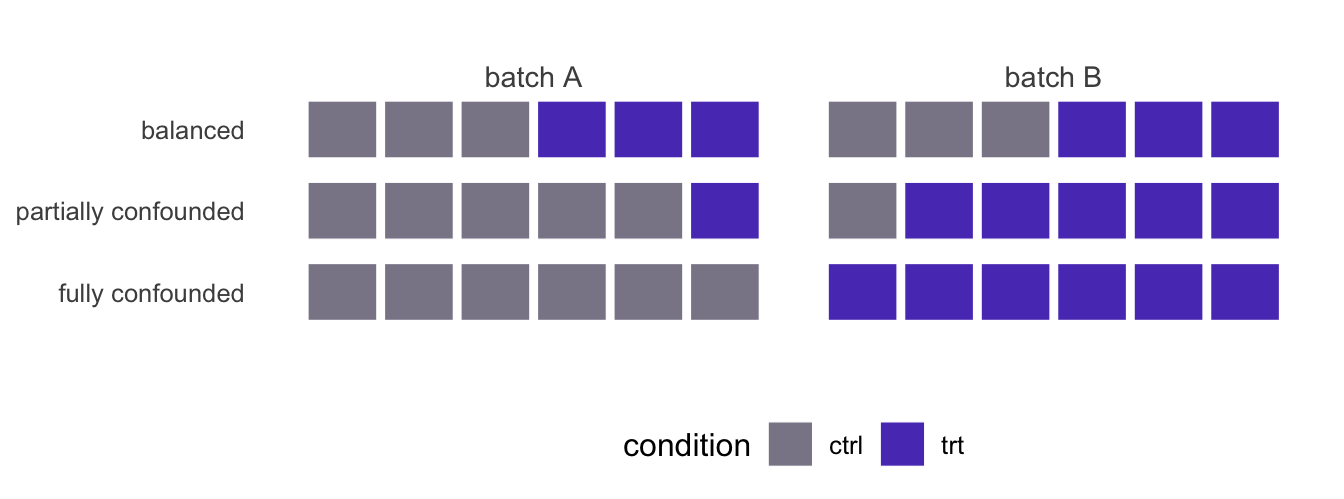
Each simulated experiment has twelve samples: six controls and six treated, processed in two batches of six. Only the allocation of samples to batches changes between the three designs.
$balanced
     condition
batch ctrl trt
    A    3   3
    B    3   3

$partial
     condition
batch ctrl trt
    A    5   1
    B    1   5

$full
     condition
batch ctrl trt
    A    6   0
    B    0   6
lay <-do.call(rbind, lapply(names(designs), function(nm) { d <- designs[[nm]]data.frame(design = nm, x =seq_len(12) + (d$batch =="B") *0.8, cond = d$cond)}))lay$design <-factor(lay$design, levels =rev(names(designs)),labels =rev(c("balanced", "partially confounded", "fully confounded")))ggplot(lay, aes(x, design, fill = cond)) +geom_tile(width =0.9, height =0.7, colour ="white") +annotate("text", x =c(3.5, 10.3), y =3.65, label =c("batch A", "batch B"),colour ="grey30", size =3.8) +scale_fill_manual(values =c(ctrl = grey, trt = violet), name ="condition") +coord_cartesian(ylim =c(0.6, 3.8)) +labs(x =NULL, y =NULL) + theme_pc +theme(axis.text.x =element_blank(), panel.grid =element_blank())
Figure 1: The three sample layouts. Each row is one experiment of twelve samples split over two batches; colour shows the condition.
The counts are negative binomial, the usual model for RNA-seq read counts, for 3,000 genes. The first 300 genes have a true change between conditions, a log2 fold change of plus or minus 1; the rest have none. Every gene also gets a batch shift, drawn once per gene from a normal distribution with a standard deviation of 0.7 on the log2 scale, so batch B moves some genes up and others down. Library sizes differ a little between samples.
Two assumptions carry the argument. The batch effect adds to the condition effect on the log scale (it is the same in control and treated samples), and the batch labels are known. These are exactly the assumptions of a ~ batch + condition model, so the model is given its best chance. The simulation is repeated 6 times; within each repeat, the three designs share the same genes and differ only in which samples sit in which batch.
G <-3000n_de <- G /10true_lfc <-1# log2 fold change of the DE genesbatch_sd <-0.7# spread of per-gene log2 batch effectssim_genes <-function() { mu0 <-exp(rnorm(G, log(150), 1.3)) # baseline mean countlist(mu0 = mu0,phi =0.03+0.3/sqrt(mu0), # NB dispersion, higher for low countslfc =c(sample(c(-1, 1) * true_lfc, n_de, TRUE), rep(0, G - n_de)),bfx =rnorm(G, 0, batch_sd)) # log2 batch B effect, every gene}sim_counts <-function(g, d) { lf <-outer(g$lfc, d$cond =="trt") +outer(g$bfx, d$batch =="B") mu <- g$mu0 *2^lf *rep(runif(12, 0.8, 1.25), each = G) m <-matrix(rnbinom(G *12, mu = mu, size =1/ g$phi), G, 12)storage.mode(m) <-"integer" m}is_de <-seq_len(G) <= n_de
Full confounding is not a statistics problem
In the fully confounded design, the column of the design matrix that marks batch B is identical to the column that marks the treated samples. The matrix has three columns but only two independent ones, and no fitting procedure can split one number into two.
the model matrix is not full rank, so the model cannot be fit as specified.
  One or more variables or interaction terms in the design formula are linear
  combinations of the others and must be removed.

  Please read the vignette section 'Model matrix not full rank':

  vignette('DESeq2')
edger_msg <-tryCatch({ y <-normLibSizes(DGEList(cts))estimateDisp(y, X_full)}, error =function(e) conditionMessage(e))cat(edger_msg)
Design matrix not of full rank.  The following coefficients not estimable:
 condtrt
# removeBatchEffect without group: what is left of the condition difference?lc_full <-cpm(DGEList(cts), log =TRUE, prior.count =3)rb_full <-removeBatchEffect(lc_full, batch = designs$full$batch,design =matrix(1, ncol(lc_full), 1))max_diff_full <-max(abs(rowMeans(rb_full[, designs$full$cond =="trt"]) -rowMeans(rb_full[, designs$full$cond =="ctrl"])))max_diff_full
[1] 7.105427e-15
# ... and with group: the warning is caught here so that it can be printedcaught <-character(0)rb_group <-withCallingHandlers(removeBatchEffect(lc_full, batch = designs$full$batch, group = designs$full$cond),warning =function(w) { caught <<-c(caught, conditionMessage(w)); invokeRestart("muffleWarning") })
Both packages refuse, and they are right to. DESeq2 stops as soon as the data object is built, with a message that the model matrix is not full rank; edgeR stops at dispersion estimation and names the coefficient it cannot estimate. limma’s nonEstimable() gives the same answer before any data are involved.
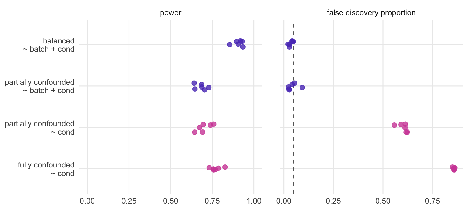
The tempting workarounds do not help. Dropping batch and fitting ~ condition runs without complaint, but the “condition” coefficient is now condition plus batch: in the simulation, 86% of the genes called at 5% FDR (false discovery rate) have no true condition effect (Figure 2). Running removeBatchEffect() on the data first is no better. Without the group argument, it removes the batch B shift, which is also the whole treatment difference: the largest remaining difference between condition means is 7.1e-15 log2 units, zero up to rounding error. With group supplied, the function reports that the batch coefficient cannot be estimated, issues a warning (caught and printed above), and returns the data unchanged: the largest change to any value is 0. Testing that output with ~ condition is the first workaround again. Batch effects are widespread in high-throughput data, and when they line up with the biological groups they lead to wrong conclusions (Leek et al. 2010).
Partial confounding: put batch in the model
In the other two designs every batch holds both conditions, so the model can estimate the batch shift from within-condition comparisons and the condition effect from within-batch comparisons. The analysis is edgeR’s quasi-likelihood pipeline (Chen et al. 2016) in its current form. Filtering uses filterByExpr(), which according to its help page implements the filtering that paper describes informally, and normalisation uses normLibSizes() (a newer name for calcNormFactors()). glmQLFit() is called with robust = TRUE, as in the paper, and with legacy = FALSE, the new quasi-likelihood method that is the default from edgeR 4.2 onwards; in that mode glmQLFit() estimates the negative binomial dispersion itself, so no separate estimateDisp() step is needed. glmQLFTest() then tests the condition coefficient.
run_edger <-function(cts, X) { y <-DGEList(cts) keep <-filterByExpr(y, X) y <-normLibSizes(y[keep, , keep.lib.sizes =FALSE]) fit <-glmQLFit(y, X, robust =TRUE, legacy =FALSE) res <-glmQLFTest(fit, coef ="condtrt")list(p = res$table$PValue, lfc = res$table$logFC, keep = keep)}score <-function(p, de) { called <-p.adjust(p, "BH") <0.05c(fpr =mean(p[!de] <0.05), # nulls with raw p < 0.05fdp =if (any(called)) mean(!de[called]) else0, # false discovery proportionpower =mean(called[de])) # true DE genes called}
The loop below runs every analysis in the post on each simulated experiment: the edgeR fits for this section, and the limma fits used in the next one.
n_rep <-6runs1 <-list(c("balanced", "~ batch + cond"), c("partial", "~ batch + cond"),c("partial", "~ cond"), c("full", "~ cond"))set.seed(2026)res1 <-list(); res2 <-list(); nullp <-list()for (r inseq_len(n_rep)) { g <-sim_genes() cts_by <-lapply(designs, function(d) sim_counts(g, d))for (k in runs1) { d <- designs[[k[1]]] e <-run_edger(cts_by[[k[1]]], model.matrix(as.formula(k[2]), d)) res1[[length(res1) +1]] <-data.frame(rep = r, design = k[1], model = k[2],t(score(e$p, is_de[e$keep]))) }# next section: limma-trend on log-CPM, batch in the model vs removeBatchEffect firstfor (nm inc("balanced", "partial")) { d <- designs[[nm]] X2 <-model.matrix(~ batch + cond, d); X1 <-model.matrix(~ cond, d) y <-DGEList(cts_by[[nm]]) keep <-filterByExpr(y, X2) y <-normLibSizes(y[keep, , keep.lib.sizes =FALSE]) lc <-cpm(y, log =TRUE, prior.count =3) fits <-list("batch in model"=eBayes(lmFit(lc, X2), trend =TRUE),"removeBatchEffect with group"=eBayes(lmFit(removeBatchEffect(lc, batch = d$batch, group = d$cond), X1), trend =TRUE),"removeBatchEffect without group"=eBayes(lmFit(removeBatchEffect(lc, batch = d$batch, design =matrix(1, ncol(lc), 1)), X1), trend =TRUE))for (m innames(fits)) { p <- fits[[m]]$p.value[, "condtrt"] lfc <- fits[[m]]$coefficients[, "condtrt"] de <- is_de[keep] res2[[length(res2) +1]] <-data.frame(rep = r, design = nm, method = m,t(score(p, de)), lfc_de =median(abs(lfc[de])))if (nm =="partial") nullp[[length(nullp) +1]] <-data.frame(method = m, p = p[!de]) } }}res1 <-do.call(rbind, res1); res2 <-do.call(rbind, res2); nullp <-do.call(rbind, nullp)agg1 <-aggregate(cbind(fpr, fdp, power) ~ design + model, res1, mean)agg2 <-aggregate(cbind(fpr, fdp, power, lfc_de) ~ design + method, res2, mean)
a1 <-function(d, m, v) agg1[agg1$design == d & agg1$model == m, v]pow_bal <-a1("balanced", "~ batch + cond", "power")pow_par <-a1("partial", "~ batch + cond", "power")fdp_bal <-a1("balanced", "~ batch + cond", "fdp")fdp_par <-a1("partial", "~ batch + cond", "fdp")fdp_par_nob <-a1("partial", "~ cond", "fdp")fdp_full <-a1("full", "~ cond", "fdp")# precision of the condition coefficient: diagonal of (X'X)^-1, in units of sigma^2vf <-sapply(designs[1:2], function(d) { X <-model.matrix(~ batch + cond, d); solve(crossprod(X))["condtrt", "condtrt"] })se_ratio <-sqrt(vf["partial"] / vf["balanced"])n_equiv <-2/ vf["partial"] # per-group n of an unconfounded design with equal precisionagg1
    design          model        fpr        fdp     power
1 balanced ~ batch + cond 0.05025914 0.03471029 0.9057948
2  partial ~ batch + cond 0.04960208 0.04436586 0.6817737
3     full         ~ cond 0.56486524 0.85723246 0.7711475
4  partial         ~ cond 0.29171683 0.60200705 0.7002244
Figure 2: Power (left) and false discovery proportion (right) for edgeR quasi-likelihood tests at a 5% FDR cut-off. Each dot is one simulated experiment; the dashed line marks the nominal 5%.
With ~ batch + condition, both designs keep the false discovery proportion close to the 5% target on average (3.5% balanced, 4.4% partially confounded). The price of the lopsided layout is power: 91% of the truly changed genes are found in the balanced design and 68% in the partially confounded one, from the same number of samples.
The loss follows from the design alone. The variance of the condition estimate is the residual variance times a factor that depends only on the design matrix (the matching diagonal entry of ). That factor is 0.33 for the balanced design and 0.60 for the partial one, so the standard error is 1.34 times larger. The only information about the treatment effect comes from comparisons inside a batch, and in batch A that means five controls against a single treated sample. Twelve samples laid out this way estimate the condition effect about as precisely as an unconfounded design with 3.3 samples per group.
Leaving batch out of the partial design is worse than a loss of power. Now the batch shift leaks into the condition estimate, and 60% of the calls are false.
Correcting first, testing later
A common shortcut is to “clean” the data once and then run the differential expression (DE) test on the result: compute log-CPM values (log counts per million), remove the batch with limma::removeBatchEffect(), and pass the corrected matrix to lmFit() with ~ condition as if it were ordinary data. The comparison uses limma (Ritchie et al. 2015) in its limma-trend form: lmFit() on the log-CPM values, then eBayes(trend = TRUE). The eBayes() help page recommends limma-trend for RNA-seq log-CPM values when library sizes are reasonably consistent, as they are here. Batch is either in the design matrix or removed beforehand. removeBatchEffect() is run two ways. With group = condition, the function fits batch and condition together and removes only the batch part, which is how its help page says to protect the effect of interest. Without group, the batch is estimated on its own.
a2 <-function(d, m, v) agg2[agg2$design == d & agg2$method == m, v]m0 <-"batch in model"; mg <-"removeBatchEffect with group"; mn <-"removeBatchEffect without group"fpr_model_par <-a2("partial", m0, "fpr"); fpr_g_par <-a2("partial", mg, "fpr")fpr_n_par <-a2("partial", mn, "fpr")fdp_model_par <-a2("partial", m0, "fdp"); fdp_g_par <-a2("partial", mg, "fdp")pow_model_par <-a2("partial", m0, "power"); pow_g_par <-a2("partial", mg, "power")pow_n_par <-a2("partial", mn, "power")lfc_model_par <-a2("partial", m0, "lfc_de"); lfc_n_par <-a2("partial", mn, "lfc_de")fpr_model_bal <-a2("balanced", m0, "fpr"); fpr_g_bal <-a2("balanced", mg, "fpr")fpr_n_bal <-a2("balanced", mn, "fpr")# with group: the naive fit uses (X1'X1)^-1 instead of the full-model variance factorX1p <-model.matrix(~ cond, designs$partial)t_inflate <-sqrt(vf["partial"] /solve(crossprod(X1p))["condtrt", "condtrt"])# without group: share of the condition contrast left after regressing on batch alonegp <-as.numeric(designs$partial$cond =="trt")keep_share <-sum(resid(lm(gp ~ designs$partial$batch))^2) /sum((gp -mean(gp))^2)# check on the last partial experiment: same estimate, one residual df more, smaller SElc_p <-cpm(normLibSizes(DGEList(cts_by$partial)), log =TRUE, prior.count =3)X2p <-model.matrix(~ batch + cond, designs$partial)fit_full <-lmFit(lc_p, X2p)fit_naive <-lmFit(removeBatchEffect(lc_p, batch = designs$partial$batch,group = designs$partial$cond), X1p)est_diff <-max(abs(fit_full$coefficients[, "condtrt"] - fit_naive$coefficients[, "condtrt"]))df_full <- fit_full$df.residual[1]; df_naive <- fit_naive$df.residual[1]agg2
    design                          method         fpr        fdp      power
1 balanced                  batch in model 0.047814449 0.02823014 0.90183235
2  partial                  batch in model 0.049665731 0.04375510 0.66448768
3 balanced    removeBatchEffect with group 0.060334592 0.04617665 0.91649528
4  partial    removeBatchEffect with group 0.162727008 0.34317329 0.89826435
5 balanced removeBatchEffect without group 0.060334592 0.04617665 0.91649528
6  partial removeBatchEffect without group 0.007460888 0.00000000 0.07046143
     lfc_de
1 0.9764442
2 0.9710172
3 0.9764442
4 0.9710172
5 0.9764442
6 0.5394540
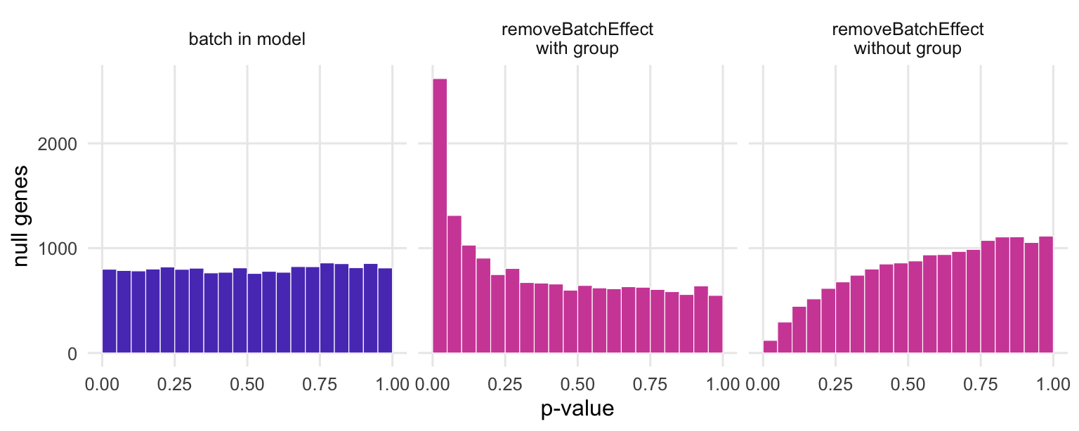
Figure 3: P-values of genes with no true condition effect in the partially confounded design, pooled over all simulated experiments. A correct test gives a flat histogram.
In the partially confounded design the two shortcuts fail in opposite directions. With batch in the model, 5.0% of the genes without a true effect have p < 0.05, as a valid test should. After removeBatchEffect() with group, that share is 16.3%, and 34% of the genes called at 5% FDR are false. The same analysis appears to find 90% of the true changes, against 66% with batch in the model; that extra power is bought with the inflated error rate, not with information.
The reason is bookkeeping. After the correction, the condition estimate is the same number the full model would give (the largest difference over all genes in the last simulated experiment is 3.8e-15), but the second fit does not know that a batch effect was estimated from these twelve samples. It computes the standard error of a plain six-against-six comparison, which is too small by the factor of 1.34 from the previous section, and it counts 10 residual degrees of freedom where the full model has 9. Each t-statistic grows by that factor, and a little more for the extra degree of freedom, so in the histogram the null p-values pile up near zero. Nygaard et al. (2016) describe this effect for batch adjustment methods that retain group differences when groups are unevenly spread across batches.
Without group, the failure is loss of signal. The batch estimate is simply the difference between batch means, and with five treated samples in batch B, part of that difference is the treatment. Subtracting it leaves 56% of the true condition difference; the median estimated absolute log2 fold change of the truly changed genes drops to 0.54, against 0.97 with batch in the model (the truth is 1). Only 7% of true changes are found, and just 0.7% of null genes reach p < 0.05.
In the balanced design, the two versions of removeBatchEffect() give identical results, because batch and condition are unrelated, and the damage is smaller: 6.0% of null genes reach p < 0.05, against 4.8% with batch in the model. The excess comes from the extra degree of freedom alone. Balance limits the harm of the shortcut but does not make it correct.
The limma documentation says as much. The help page for removeBatchEffect() (limma 3.66.0, the version used here) describes it as a tool for plotting and exploration, such as PCA, MDS plots or heatmaps. Its note states that it is not meant to prepare data for linear modelling with lmFit(), and that batch factors should go into the linear model so that the standard errors are assessed correctly.
What to do in practice
Fix the layout before the samples are processed. Spread every condition over every batch, as evenly as the sample numbers allow. If extraction or library preparation has to happen over several days, each day should include samples from each group. Check the layout from the sample sheet before sequencing:
table(samples$batch, samples$condition) # every cell should be non-zeroX <-model.matrix(~ batch + condition, samples)limma::nonEstimable(X) # NULL means every coefficient can be estimated
Analyse with batch in the design formula, in whichever package you use:
Use removeBatchEffect() for pictures only, with the design so that the condition difference stays visible, and keep the uncorrected counts for testing:
If the design is already fully confounded, no software step can recover the condition effect; the honest report says so. Adding new samples of each condition to the other batch turns it into a partially confounded design, which the model can analyse. Re-processing the same biological samples does not count as new samples: repeated libraries of one sample are technical replicates and must be handled as such (for example summed with edgeR::sumTechReps()), not added as independent replicates.
References
Leek JT, Scharpf RB, Corrada Bravo H et al. 2010 Nature Reviews Genetics 11(10):733-739 (doi:10.1038/nrg2825)