How to read and test a DESeq2 interaction term, why significant in one genotype but not the other is not a difference, and how to get each genotype’s effect.
You have two genotypes, a treatment, and RNA-seq counts from every combination. Which genes respond to the treatment differently in the two genotypes? A common answer is to analyse each genotype on its own and call a gene “genotype-specific” when it is significant in one analysis and not in the other. The correct answer is a single model with an interaction term, ~ genotype + treatment + genotype:treatment, and a test of the interaction coefficient. In the simulation below, the two-list approach labels 29% of the genes that respond identically in both genotypes as genotype-specific, and 29.3% of all its genotype-specific calls are genes with no true difference in response. For the interaction test that share is 5.1%, about the 5% target.
What the interaction coefficient is
The experiment has two factors with two levels each: genotype A or B, control or treated. That gives four groups of samples. DESeq2 fits a negative binomial generalised linear model to each gene; its coefficients are on the log2 scale, so each one other than the intercept is a log2 fold change (Love et al. 2014). With the interaction in the design formula there are four coefficients for the four group means:
cd <-data.frame(genotype =factor(rep(c("A", "B"), each =6)),treatment =factor(rep(rep(c("ctrl", "trt"), each =3), 2)))table(cd$genotype, cd$treatment)
Read them with genotype A and control as the reference levels (the first level of each factor). The intercept is the log2 mean of untreated genotype A. genotypeB is the difference between the genotypes in untreated samples. treatmenttrt is the treatment effect in genotype A only, not an average over genotypes; the DESeq2 vignette calls this the key point to remember about designs with interaction terms. The interaction, genotypeB:treatmenttrt, is the treatment effect in genotype B minus the treatment effect in genotype A. A gene that goes up fourfold with treatment in A (log2 fold change 2) and twofold in B (log2 fold change 1) has an interaction of minus 1. The treatment effect in B is the sum of the treatment coefficient and the interaction.
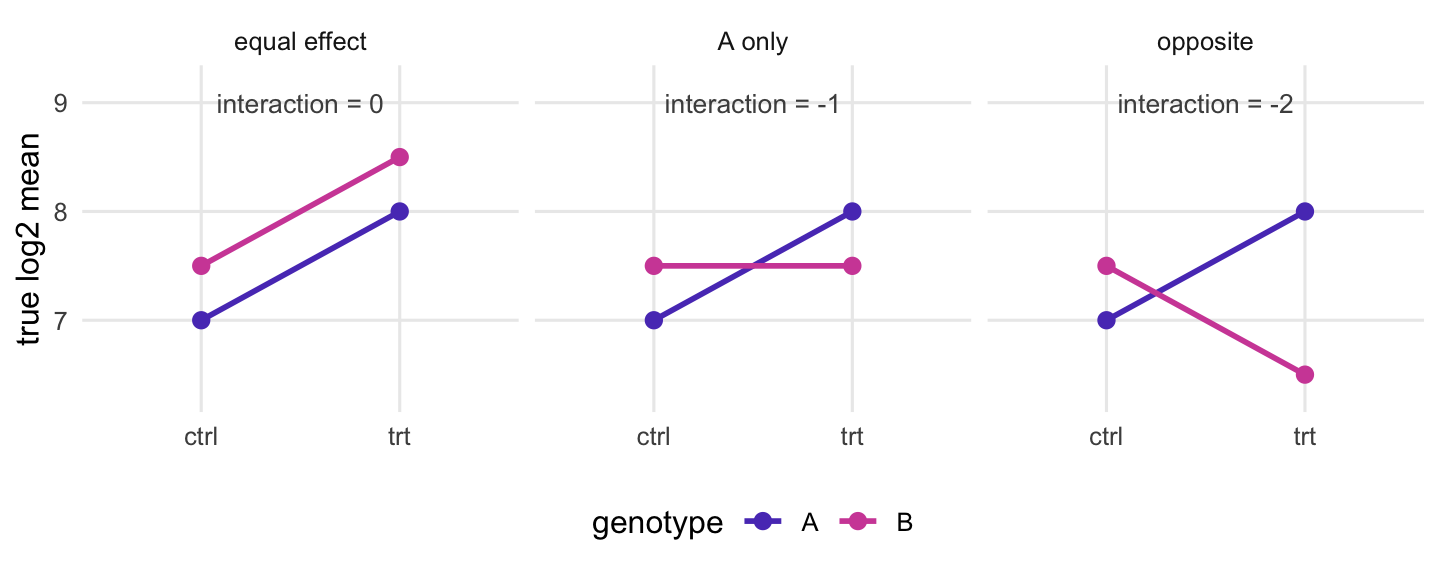
So the interaction coefficient answers exactly the question “does the treatment response differ between genotypes?”, and its test is the test of that question. The figure shows the three patterns used below.
ex <-expand.grid(treatment =c("ctrl", "trt"), genotype =c("A", "B"),type =c("equal effect", "A only", "opposite"))slope <-c("equal effect"=1, "A only"=0, "opposite"=-1) # effect in B for an effect of 1 in Aex$log2mu <-7+0.5* (ex$genotype =="B") + (ex$treatment =="trt") *ifelse(ex$genotype =="A", 1, slope[as.character(ex$type)])lab <-data.frame(type =factor(names(slope), levels =levels(ex$type)),txt =paste("interaction =", slope -1))ggplot(ex, aes(treatment, log2mu, colour = genotype, group = genotype)) +geom_line(linewidth =1) +geom_point(size =2.5) +geom_text(data = lab, aes(x =1.5, y =9, label = txt), inherit.aes =FALSE,colour ="grey30", size =3.5) +facet_wrap(~ type) +coord_cartesian(ylim =c(6.3, 9.2)) +scale_colour_manual(values =c(A = violet, B = magenta)) +labs(x =NULL, y ="true log2 mean") + theme_pc
Figure 1: Schematic of the three kinds of treatment response in the simulation (illustrative values). Each panel is one gene type; lines join the control and treated means of each genotype. The interaction coefficient is the difference between the two slopes.
The simulation
Each simulated experiment has twelve samples, three per group, and 3,000 genes. Counts are negative binomial, the usual model for RNA-seq read counts, with more scatter for weakly expressed genes. Every gene gets its own baseline level and a random baseline difference between the genotypes. The genes fall into four types:
1,800 genes do not respond to the treatment in either genotype;
400 respond with the same log2 fold change in both genotypes;
400 respond in genotype A and not at all in B;
400 respond in A and by the same amount in the opposite direction in B.
For the responding genes the size of the log2 fold change is drawn between 0.6 and 1.4, with a random sign. Only the last two types have a true interaction.
G <-3000n_cls <-c(null =1800, equal =400, A_only =400, opposite =400)cls <-factor(rep(names(n_cls), n_cls), levels =names(n_cls))lfc_range <-c(0.6, 1.4) # |log2 fold change| of responding genessim_genes <-function() { mu0 <-exp(rnorm(G, log(150), 1.3)) # baseline mean count d <-runif(G, lfc_range[1], lfc_range[2]) *sample(c(-1, 1), G, TRUE) bA <-ifelse(cls =="null", 0, d) # treatment effect in genotype A bB <-ifelse(cls %in%c("null", "A_only"), 0, # treatment effect in genotype Bifelse(cls =="equal", d, -d))list(mu0 = mu0, phi =0.03+0.3/sqrt(mu0), # NB dispersion, higher for low countsbA = bA, bB = bB, gx =rnorm(G, 0, 0.5)) # gx: genotype B baseline shift}sim_counts <-function(g) { isB <- cd$genotype =="B"; isT <- cd$treatment =="trt" lf <-outer(g$gx, isB) +outer(g$bA, isT &!isB) +outer(g$bB, isT & isB) mu <- g$mu0 *2^lf *rep(runif(12, 0.8, 1.25), each = G) m <-matrix(rnbinom(G *12, mu = mu, size =1/ g$phi), G, 12)storage.mode(m) <-"integer" m}
The size of the problem shown below depends on power, the chance that a truly responding gene reaches significance. If power were close to 1 or close to 0, the two-list approach would rarely split a gene. It does the most damage in between, which is where this three-replicate experiment with moderate effects sits. The other assumptions (balanced groups, effects that add on the log scale, a correct count model) are shared by both analyses.
Each dataset is analysed in two ways, both with the DESeq2 standard workflow (DESeq(), then results() at a 5% false discovery rate, FDR, with its alpha argument set to that cut-off as the vignette asks whenever the cut-off differs from the default). The first fits one model to all twelve samples and tests the interaction coefficient. The second splits the samples by genotype, fits ~ treatment to each half, and compares the two lists of significant genes, which is what a Venn diagram of the two lists does.
alpha <-0.05# FDR cut-offsig <-function(r) !is.na(r$padj) & r$padj < alphaanalyse <-function(cts) {# one model with the interaction dds <-DESeq(DESeqDataSetFromMatrix(cts, cd, ~ genotype + treatment + genotype:treatment),quiet =TRUE) inter <-results(dds, name ="genotypeB.treatmenttrt", alpha = alpha) inA <-results(dds, name ="treatment_trt_vs_ctrl", alpha = alpha) inB <-results(dds, contrast =list(c("treatment_trt_vs_ctrl", "genotypeB.treatmenttrt")),alpha = alpha)# two separate analyses, one per genotype sep <-lapply(c(A ="A", B ="B"), function(k) { s <- cd$genotype == k d <-DESeq(DESeqDataSetFromMatrix(cts[, s], cd[s, ], ~ treatment), quiet =TRUE)results(d, name ="treatment_trt_vs_ctrl", alpha = alpha) })list(dds = dds, inter = inter, inA = inA, inB = inB, sepA = sep$A, sepB = sep$B)}
The loop repeats the whole experiment 5 times with new genes and new counts. For every repeat it records, per gene type, the share of genes each approach calls genotype-dependent.
n_rep <-5set.seed(2026)rates <-list()for (r inseq_len(n_rep)) { g <-sim_genes() cts <-sim_counts(g) a <-analyse(cts)if (r ==1) { g1 <- g; cts1 <- cts; a1 <- a } sA <-sig(a$sepA); sB <-sig(a$sepB) venn <-xor(sA, sB) # significant in one genotype only venn1 <-xor(sig(a$inA), sig(a$inB)) # the same, from the one-model contrasts inter <-sig(a$inter) diff_true <- g$bA != g$bB rates[[r]] <-data.frame(rep = r, class =levels(cls),venn =tapply(venn, cls, mean), venn1 =tapply(venn1, cls, mean),inter =tapply(inter, cls, mean), both =tapply(sA & sB, cls, mean),sigA =tapply(sA, cls, mean), sigB =tapply(sB, cls, mean),fdp_venn =mean(!diff_true[venn]), fdp_venn1 =mean(!diff_true[venn1]),fdp_inter =mean(!diff_true[inter]), n_venn =sum(venn), n_inter =sum(inter),se_ratio =median(a$inter$lfcSE / a$inA$lfcSE, na.rm =TRUE))}rates <-do.call(rbind, rates)
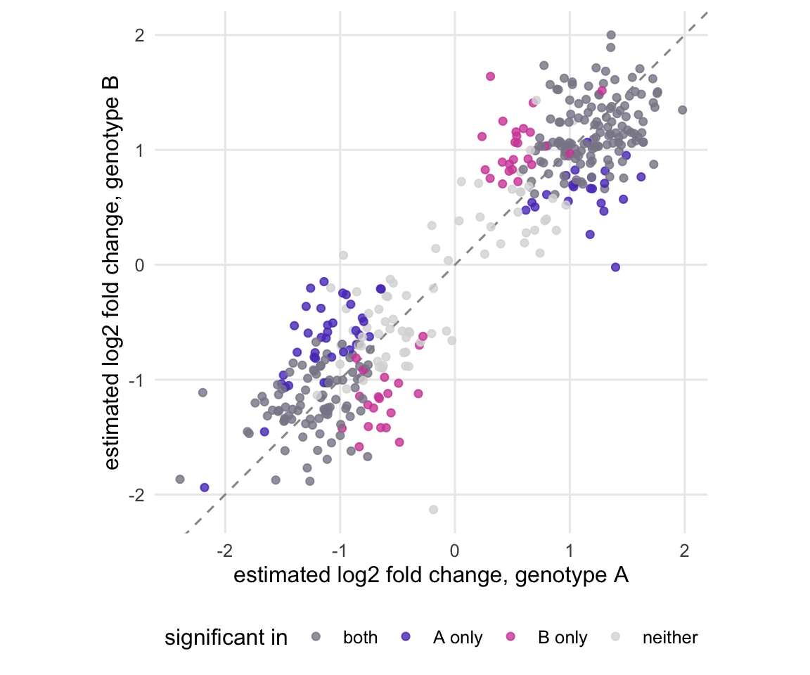
In the separate analyses, 70% of the equal-effect genes are significant in genotype A and 65% in genotype B. Those are two imperfect detectors pointed at the same signal, and they often disagree: 29% of the equal-effect genes are significant in exactly one genotype (between 26% and 31% across the repeats), and a Venn diagram puts every one of them in a genotype-specific segment. The next figure shows these genes for the first simulated experiment.
Figure 2: Estimated treatment log2 fold changes from the two separate analyses, for the genes whose true effect is the same in both genotypes (first simulated experiment). Colour shows the Venn label; the diagonal is equal effect.
The coloured points are not spread at random. Genes called in genotype A only sit on the A side of the diagonal, with a larger estimated effect in A than in B, and genes called in B only sit on the B side; in this experiment that holds for 98% of them. They form the edges of the same clouds as the grey genes. That is selection, not biology. A gene lands in the A-only segment when noise pushes its estimate in A over the significance threshold and its estimate in B below it, so the genes in that segment are the ones whose two estimates happened to drift apart. The median gap between the two estimated log2 fold changes is 0.47 for the genes significant in one genotype only, against 0.23 for the genes significant in both.
A reader looking at the figure could take that wider gap as evidence of a different response. It is not: the true effects are identical, and the gap is no larger than the noise in two separate estimates produces. The interaction test, which asks exactly whether the two effects differ, flags 1 of the 104 genes in this experiment that the Venn diagram puts in a genotype-specific segment. Gelman and Stern (2006) put the general point in their title: the difference between “significant” and “not significant” is not itself statistically significant. A non-significant result in genotype B means the data could not show an effect there, not that there is none.
The error is not caused by fitting the two genotypes separately. Taking the two per-genotype effects from the single interaction model (shown further down) and comparing their significance calls in the same way labels 27% of the equal-effect genes as genotype-specific, and 29% of those calls are false. The problem is the comparison of two significance calls, wherever they come from.
The two-list approach also mislabels many of the most striking genes. Of the genes that respond in opposite directions, 54% are significant in both analyses. In a Venn diagram of gene identifiers they sit in the shared segment, as “responds in both genotypes”, although the response is reversed. Only 28% of them are called genotype-specific. Splitting the lists by direction of change catches these genes, but not the equal-effect problem above.
The interaction test
long <-rbind(data.frame(rates[, c("rep", "class")], method ="Venn of two analyses", value = rates$venn),data.frame(rates[, c("rep", "class")], method ="interaction test", value = rates$inter))long$class <-factor(long$class, levels =rev(levels(cls)),labels =rev(c("null", "equal effect", "A only", "opposite")))long$y <-as.numeric(long$class) +ifelse(long$method =="interaction test", 0.15, -0.15)ggplot(long, aes(value, y, colour = method)) +geom_point(size =2.4, alpha =0.8) +scale_colour_manual(values =c("Venn of two analyses"= magenta, "interaction test"= violet),name =NULL) +scale_y_continuous(breaks =seq_along(levels(long$class)), labels =levels(long$class)) +coord_cartesian(xlim =c(0, 1)) +labs(x ="share of genes called genotype-dependent", y =NULL) + theme_pc
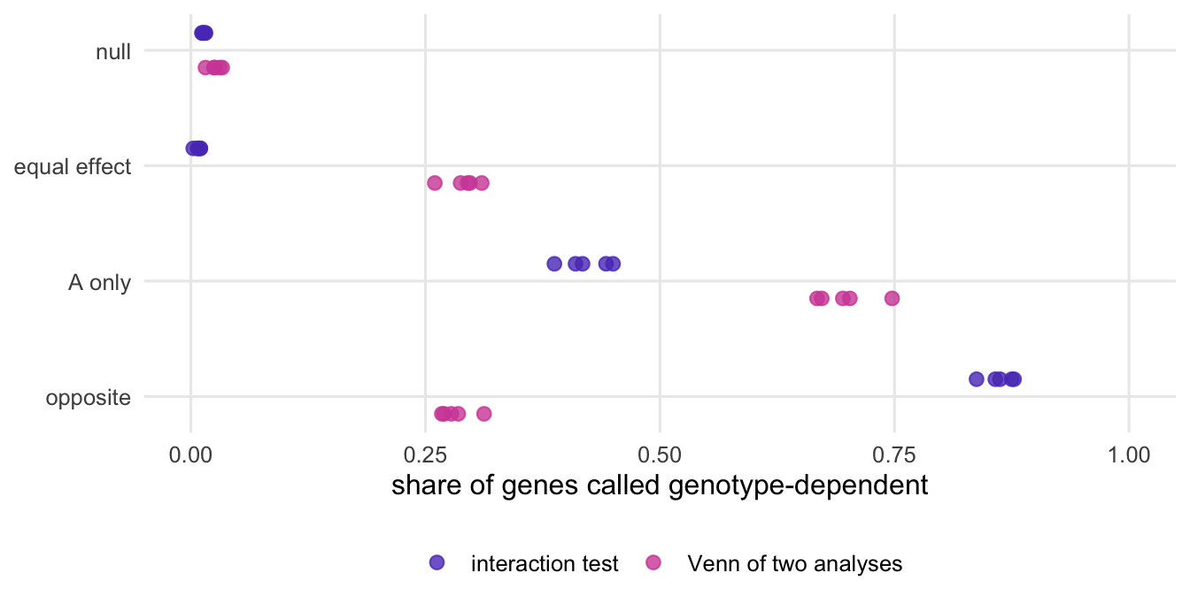
Figure 3: Share of genes called genotype-dependent by the Venn approach (significant in one separate analysis only) and by the interaction test (adjusted p below the FDR cut-off), by true response type. Each dot is one simulated experiment.
The interaction test calls 0.8% of the equal-effect genes and 1.4% of the non-responding genes genotype-dependent. Among all genes it calls, 5.1% have no true interaction on average (between 4.3% and 6.0% across the repeats), about the 5% target it was run at (a little above it in some repeats). For the two-list approach the same share is 29.3% on average. Both lists are about the same length, 541 genes for the interaction test and 554 for the Venn approach; they differ in what is on them. The interaction test also finds 86% of the opposite-direction genes.
There is a cost, and the figure shows it. For genes that respond in genotype A only, the interaction test finds 42%, while the two-list approach labels 70% of them genotype-specific. That is not extra power in the two-list approach. It applies a lower bar (significant in one genotype, not in the other), and the same lower bar is what mislabels the equal-effect genes; a list that cannot tell you which 29.3% of its entries are wrong is not a better list.
The interaction really is harder to estimate than a single treatment effect. It is a difference between two differences, each estimated from six samples, so its variance is the sum of theirs. In this balanced design the standard error of the interaction coefficient is 1.41 times that of the treatment effect in one genotype (the square root of 2, from the design matrix alone); the median ratio of the standard errors DESeq2 reports is 1.42. To detect a given difference in response with the same power as a response of the same size within one genotype, the sample size has to grow by a factor of about 2, and by more if the difference in response you care about is smaller than the response itself. If a genotype-dependent response is the main question of the experiment, that belongs in the sample size calculation.
The treatment effect in each genotype
Often you want the per-genotype effects as well, for example to report a fold change for each genotype next to the interaction test. All of them come from the one model. The names DESeq2 gives the coefficients differ from the model matrix column names (the main effects are renamed and the colon becomes a dot), so read them off resultsNames() rather than typing them from memory:
# argument names used belowc("name", "contrast", "alpha") %in%names(formals(results))
[1] TRUE TRUE TRUE
formals(results)$alpha # default FDR target of results()
[1] 0.1
c("test", "reduced") %in%names(formals(DESeq))
[1] TRUE TRUE
The treatment effect in genotype A is the coefficient treatment_trt_vs_ctrl, extracted with results(dds, name = "treatment_trt_vs_ctrl"). The effect in genotype B is that coefficient plus the interaction. results() accepts a list for its contrast argument; according to its help page the first element names the coefficients that are added up for the numerator, and a list of length one is completed with an empty denominator. This is the route shown in Examples 2 and 3 of the results() help page:
The chunk below checks it three ways on the first simulated dataset: against the sum of the two fitted coefficients, against a refit with genotype B as the reference level, and against the combined-factor design (~ group, with levels such as Bctrl and Btrt) that the DESeq2 vignette suggests when only per-group comparisons are wanted.
b <-coef(a1$dds) # MLE coefficients, log2 scalesum_coef <- b[, "treatment_trt_vs_ctrl"] + b[, "genotypeB.treatmenttrt"]diff_sum <-max(abs(a1$inB$log2FoldChange - sum_coef), na.rm =TRUE)# the same effect with genotype B as the reference leveldds_B <- a1$ddsdds_B$genotype <-relevel(dds_B$genotype, "B")dds_B <-DESeq(dds_B, quiet =TRUE)rB_relevel <-results(dds_B, name ="treatment_trt_vs_ctrl")diff_relevel <-max(abs(a1$inB$log2FoldChange - rB_relevel$log2FoldChange), na.rm =TRUE)diff_relevel_p <-max(abs(a1$inB$pvalue - rB_relevel$pvalue), na.rm =TRUE)# the combined-factor route from the vignettedds_g <- a1$ddsdds_g$group <-factor(paste0(dds_g$genotype, dds_g$treatment))design(dds_g) <-~ groupdds_g <-DESeq(dds_g, quiet =TRUE)rB_group <-results(dds_g, contrast =c("group", "Btrt", "Bctrl"))diff_group <-max(abs(a1$inB$log2FoldChange - rB_group$log2FoldChange), na.rm =TRUE)# the interaction as a single contrast in the ~ group designresultsNames(dds_g)
The list contrast equals the sum of the coefficients to machine precision (largest difference 4e-16). The refit with genotype B as reference and the combined-factor design give the same log2 fold changes up to the tolerance of the fitting algorithm (largest differences 5e-06 and 8e-06), and the relevelled fit gives the same p-values to within 1e-06.
The ~ group design does not take the interaction test away, although its separate per-group tables invite the Venn comparison. The interaction is the treated-minus-control difference in B minus the same difference in A, which is one list contrast of the group coefficients:
In the chunk above it reproduces the interaction coefficient of the first model (largest difference in log2 fold change 2e-05, in p-value 1e-06).
What to do in practice
When the question is whether a response differs between groups, put that question into the design formula and test the coefficient that answers it. This is the same rule as for batch effects (see the post on confounded batches): the comparison belongs in the model, not in a comparison of two results tables after the fact.
dds <-DESeqDataSetFromMatrix(counts, samples,design =~ genotype + treatment + genotype:treatment)dds$genotype <-relevel(dds$genotype, "A") # set reference levels before DESeq()dds$treatment <-relevel(dds$treatment, "ctrl")dds <-DESeq(dds)resultsNames(dds)res_diff <-results(dds, name ="genotypeB.treatmenttrt", alpha =0.05) # does the response differ?res_A <-results(dds, name ="treatment_trt_vs_ctrl", alpha =0.05) # response in genotype Ares_B <-results(dds, contrast =list(c("treatment_trt_vs_ctrl","genotypeB.treatmenttrt")),alpha =0.05) # response in genotype B
Report genes as genotype-dependent only when res_diff calls them, and show the two per-genotype fold changes side by side, with their standard errors, rather than as a Venn diagram. For plotting or ranking those fold changes, the DESeq2 vignette recommends shrunken estimates from lfcShrink(). Its default apeglm method needs a coefficient name (coef) rather than a contrast, so the effect in genotype B comes from a fit with B as the reference level:
With more than two genotypes, a likelihood ratio test asks whether the response differs anywhere: DESeq(dds, test = "LRT", reduced = ~ genotype + treatment). A gene significant in one genotype and not in the other has not been shown to be genotype-specific; it may only have been measured with less certainty in one of them.