Log2 fold change cut-off after padj: what is the FDR?
DESeq2
edgeR
limma
FDR
RNA-seq
Is padj < 0.05 plus a log2 fold change cutoff a test of a 2-fold change? A simulation against lfcThreshold in DESeq2, glmTreat in edgeR and treat in limma.
Author
Pseudocount
Published
27 September 2026
Setup: packages and helper functions
suppressPackageStartupMessages({library(DESeq2)library(apeglm)library(edgeR)library(limma)library(ggplot2)})stopifnot(packageVersion("DESeq2") >="1.40", packageVersion("apeglm") >="1.20",packageVersion("edgeR") >="4.0.0", packageVersion("limma") >="3.56",packageVersion("ggplot2") >="3.4.0")pct <-function(x, d =1) sprintf(paste0("%.", d, "f%%"), 100* x)num <-function(x) format(round(x), big.mark =",", scientific =FALSE, trim =TRUE)dec <-function(x, d =2) sprintf(paste0("%.", d, "f"), x)violet <-"#5a3fc0"; magenta <-"#d14fa6"; grey <-"#8e8c9c"; dark <-"#5f5c70"theme_set(theme_minimal(base_size =12) +theme(panel.grid.minor =element_blank(), strip.text =element_text(face ="bold"),plot.background =element_rect(fill ="white", colour ="white")))thr <-1# the size claim: |true log2 fold change| > 1, a 2-fold changealpha <-0.05# FDR level for every list in this post# score one list of calls against the truth; a call is false for the size claim when the# true change is at or below the threshold t, or when the estimate has the wrong signscore <-function(call, est, true_lfc, t = thr) { call[is.na(call)] <-FALSE right <-abs(true_lfc) > t &sign(est) ==sign(true_lfc) right[is.na(right)] <-FALSEc(n_call =sum(call),fdp =if (any(call)) mean(!right[call]) else0, # false for the size claimfdp_zero =if (any(call)) mean(true_lfc[call] ==0) else0, # false for "it changed"power =sum(call & right) /sum(abs(true_lfc) > t)) # share of big changes found}# DESeq2's two threshold tests for |LFC| > thr, from the Wald estimate and its standard errorp_thr_2014 <-function(b, se) pmin(1, 2*pnorm((abs(b) - thr) / se, lower.tail =FALSE))p_thr_new <-function(b, se) pnorm(-abs(b) + thr, sd = se) +pnorm(-abs(b) - thr, sd = se)# the p-values then go through DESeq2's own independent filtering and BH, as in results()deseq_adjust <-function(res, p) { res$pvalue <-ifelse(is.na(res$pvalue), NA_real_, p) # keep results()'s missing values DESeq2:::pvalueAdjustment(res, independentFiltering =TRUE, alpha = alpha,pAdjustMethod ="BH")$padj}# defaults quoted in the text, read from the installed packagesres_thr_default <-eval(formals(DESeq2::results)$lfcThreshold)res_alt_default <-eval(formals(DESeq2::results)$altHypothesis)[1]deseq_version <-as.character(packageVersion("DESeq2"))has_2014 <-"greaterAbs2014"%in%eval(formals(DESeq2::results)$altHypothesis) # DESeq2 >= 1.44treat_null_default <-eval(formals(edgeR::glmTreat)$null)treat_lfc_default <-eval(formals(edgeR::glmTreat)$lfc)limma_fc_default <-eval(formals(limma::treat)$fc)
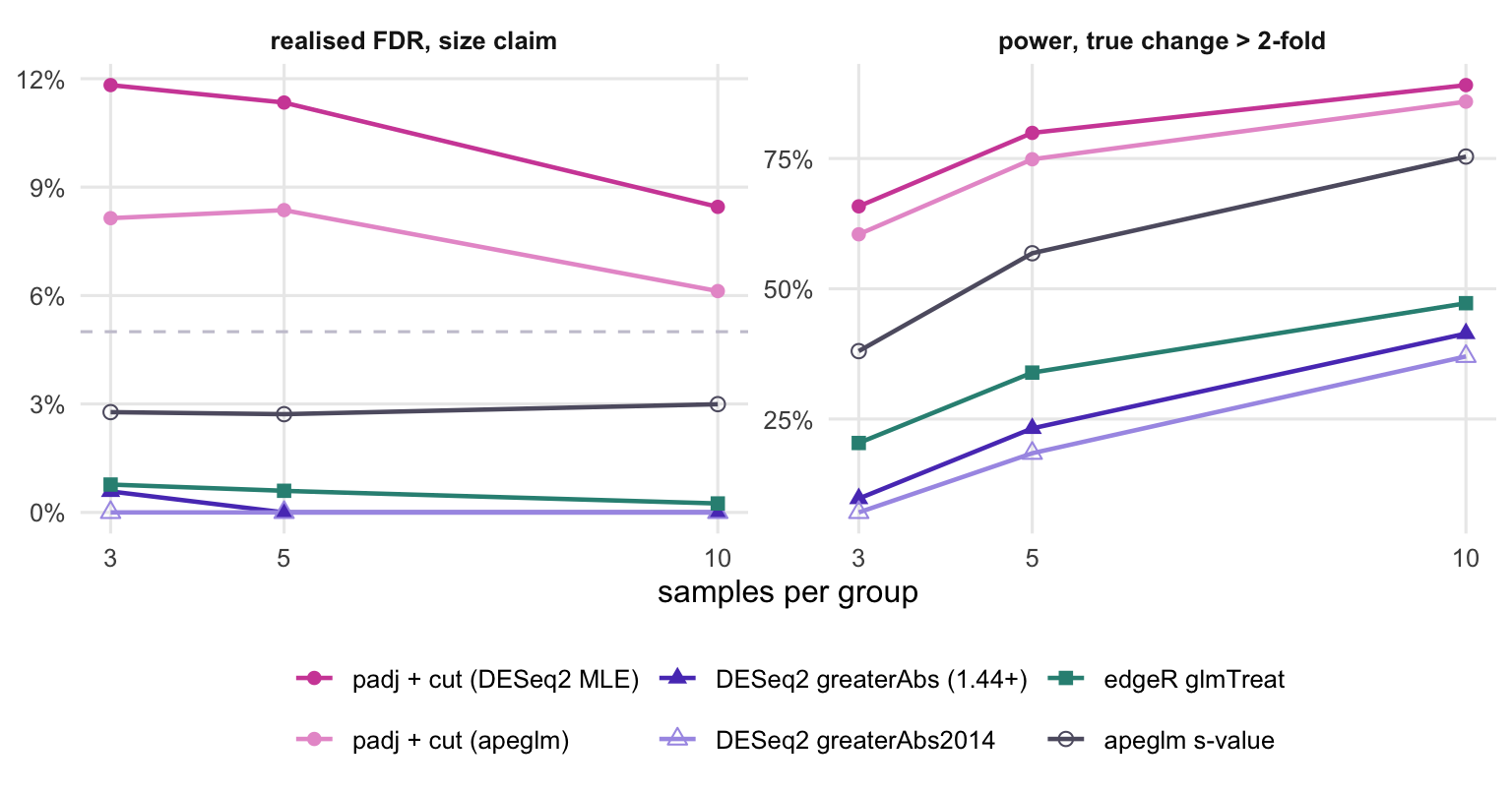
You ran DESeq2, kept the genes with padj < 0.05, and then kept those with an absolute log2 fold change above 1. The list now reads as “genes that changed more than 2-fold, at 5% FDR”. Is that what it is? No. The adjusted p-value tested whether the change is zero; the cut-off was applied to an estimate afterwards, and nothing controls how many of the genes that pass it truly changed less than 2-fold. In the simulation below, with 3 samples per group, 11.8% of the genes on such a list had a true change of 2-fold or less, for a nominal 5%. Testing against the threshold with results(dds, lfcThreshold = 1) (DESeq2 1.44 or later) kept that share at 0.6%, and paid for it in genes found: it recovered 9.7% of the genes that truly changed more than 2-fold, against 65.8% for the cut.
The setup
Each simulated dataset has 2,500 genes measured in two groups, with 3, 5 or 10 samples per group. Counts are drawn from a negative binomial distribution (the usual model for RNA-seq counts, in which the variance grows faster than the mean), with mean counts spread over several orders of magnitude and a larger dispersion, the biological part of the variance, for weakly expressed genes.
The true changes are the assumption that matters. 40% of genes change, and the size of each change, as an absolute log2 fold change, is spread evenly between 0 and 2; the sign is random. So among the genes that change, half change by less than 2-fold and half by more, and there is as much true change just below the cut-off as just above it. A call counts as false when the gene’s true absolute log2 fold change is 1 or less. That is the claim a list filtered at 1 makes, and it is stricter than “the gene changed”. A later section varies how many of the changes sit below the cut-off, because that share decides how bad the problem is.
For each sample size I simulate 4 datasets and report averages over them, since the false discovery rate (FDR) is itself an average over experiments; the table at the end also gives the range over the datasets. The datasets of one sample size are rows of one count matrix, so they share their samples’ sequencing depths (size factors).
n_values <-c(3, 5, 10) # samples per groupn_genes <-2500# genes per datasetn_exp <-4# datasets per sample sizep_change <-0.4# share of genes with a true changelfc_max <-2# |true log2 fold change| of changed genes ~ Uniform(0, lfc_max)simulate <-function(n_rows, n_per, lfc_max) { mu0 <-exp(rnorm(n_rows, log(40), 1.6)) # mean count phi <- (0.04+0.2/sqrt(mu0 +1)) *exp(rnorm(n_rows, 0, 0.3)) # dispersion changed <-runif(n_rows) < p_change lfc <-ifelse(changed, sample(c(-1, 1), n_rows, TRUE) *runif(n_rows, 0, lfc_max), 0) grp <-rep(0:1, each = n_per) size_factor <-exp(rnorm(2* n_per, 0, 0.15)) mu <-outer(mu0, size_factor) *2^outer(lfc, grp) counts <-matrix(as.integer(rnbinom(length(mu), mu = mu, size =1/ phi)), nrow = n_rows)list(counts = counts, lfc = lfc)}
Each dataset goes through three packages, each run the way its documentation describes. DESeq2 runs DESeq() and results() (Love, Huber and Anders 2014), plus lfcShrink() with the apeglm prior (Zhu, Ibrahim and Love 2019). To save time, the datasets of one sample size are stacked and run through DESeq() together (they share the fitted dispersion trend), and each is then passed to results() and lfcShrink(), filtered, corrected and scored on its own. edgeR runs its quasi-likelihood recipe: filterByExpr(), normLibSizes(), glmQLFit() with legacy = FALSE set explicitly (so that older and newer edgeR releases fit the same model), then either glmQLFTest() or glmTreat(). limma runs voom on the same filtered and normalised counts, then lmFit() and treat(). DESeq2’s threshold test changed between versions (more on this below), so the chunk computes both versions of it by hand from the Wald estimate and its standard error, and passes the p-values through DESeq2’s own independent filtering and correction, the internal function results() uses. It also checks the hand computation against results().
# all the ways of calling "more than 2-fold" genes in one datasetanalyse <-function(dds_e, counts, group, design) { r0 <-results(dds_e, alpha = alpha) # H0: LFC = 0 b <- r0$log2FoldChange; se <- r0$lfcSE p_old <-p_thr_2014(b, se); p_new <-p_thr_new(b, se)# what results() itself returns for "greaterAbs" in the installed DESeq2 (checked below) rt <-results(dds_e, lfcThreshold = thr, altHypothesis ="greaterAbs", alpha = alpha) sh <-suppressMessages( # prints a note on FSOSlfcShrink(dds_e, coef =2, type ="apeglm", lfcThreshold = thr, quiet =TRUE)) y <-DGEList(counts, group = group) keep <-filterByExpr(y, group = group) y <-normLibSizes(y[keep, , keep.lib.sizes =FALSE]) fit <-glmQLFit(y, design, robust =TRUE, legacy =FALSE) qlf <-glmQLFTest(fit, coef =2)$table tr1 <-glmTreat(fit, coef =2, lfc = thr)$table tr1w <-glmTreat(fit, coef =2, lfc = thr, null ="worst.case")$table tr15 <-glmTreat(fit, coef =2, lfc =log2(1.5))$table v <-voom(y, design) lf <-lmFit(v, design) lt1 <-topTreat(treat(lf, lfc = thr), coef =2, number =nrow(lf), sort.by ="none") lt15 <-topTreat(treat(lf, lfc =log2(1.5)), coef =2, number =nrow(lf), sort.by ="none") full <-function(x) { out <-rep(NA_real_, length(keep)); out[keep] <- x; out } # back to all genes bh <-function(p) full(p.adjust(p, "BH")) padj_new <-deseq_adjust(r0, p_new)# each entry: the calls, the estimate whose sign is claimed, the threshold of the claim calls <-list(deseq_zero =list(r0$padj < alpha, b),deseq_post =list(r0$padj < alpha &abs(b) > thr, b),deseq_ape =list(r0$padj < alpha &abs(sh$log2FoldChange) > thr, sh$log2FoldChange),edger_post =list(bh(qlf$PValue) < alpha &full(abs(qlf$logFC)) > thr, full(qlf$logFC)),deseq_thr =list(padj_new < alpha, b),deseq_2014 =list(deseq_adjust(r0, p_old) < alpha, b),edger_thr =list(bh(tr1$PValue) < alpha, full(tr1$logFC)),edger_wc =list(bh(tr1w$PValue) < alpha, full(tr1w$logFC)),limma_thr =list(full(lt1$adj.P.Val) < alpha, full(lt1$logFC)),edger_small =list(bh(tr15$PValue) < alpha &full(abs(tr15$logFC)) > thr, full(tr15$logFC)),limma_small =list(full(lt15$adj.P.Val) < alpha &full(abs(lt15$logFC)) > thr, full(lt15$logFC)),ape_sval =list(sh$svalue < alpha, sh$log2FoldChange),edger_own15 =list(bh(tr15$PValue) < alpha, full(tr15$logFC), log2(1.5)),limma_own15 =list(full(lt15$adj.P.Val) < alpha, full(lt15$logFC), log2(1.5)))list(calls = calls,est =data.frame(mle = b, se = se, padj = r0$padj),# does the formula above reproduce results()? compare with the method it has as greaterAbscheck =max(abs(rt$padj -deseq_adjust(r0, if (has_2014) p_new else p_old)), na.rm =TRUE),p_one =c(old =mean(p_old[!is.na(r0$pvalue)] ==1), new =mean(p_new[!is.na(r0$pvalue)] ==1)),filtered =mean(!keep))}methods <-c("deseq_post", "deseq_ape", "edger_post", "deseq_thr", "deseq_2014", "edger_thr","edger_wc", "limma_thr", "edger_small", "limma_small", "ape_sval")# simulate n_exp datasets, run DESeq() once on the stack, analyse and score each datasetrun_setting <-function(n_per, lfc_max, which = methods) { group <-factor(rep(c("A", "B"), each = n_per)) design <-model.matrix(~ group) sim <-simulate(n_genes * n_exp, n_per, lfc_max) dds <-DESeqDataSetFromMatrix(sim$counts, data.frame(group = group), ~ group) dds <-DESeq(dds, quiet =TRUE)lapply(seq_len(n_exp), function(e) { i <- (e -1) * n_genes +seq_len(n_genes) a <-analyse(dds[i, ], sim$counts[i, ], group, design) sc <-t(sapply(a$calls, function(x)score(x[[1]], x[[2]], sim$lfc[i], if (length(x) >2) x[[3]] else thr)))list(scores = sc[unique(c(which, "deseq_zero", "edger_own15", "limma_own15")), ],est =cbind(a$est, true = sim$lfc[i], called = a$calls$deseq_post[[1]] %in%TRUE),check = a$check, p_one = a$p_one, filtered = a$filtered) })}
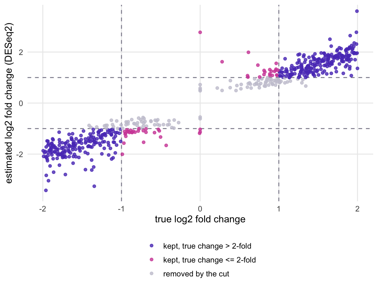
The first figure shows one dataset with 5 samples per group. Every point is a gene with padj < 0.05 from the standard DESeq2 test against zero, placed by its true log2 fold change (horizontal) and its estimate (vertical). The genes kept by the cut are the ones outside the horizontal lines. The false ones, for the size claim, are those kept although their true change lies between the vertical lines.
Figure 1: True against estimated log2 fold change in one simulated dataset, five samples per group, for genes with padj below 0.05 in the DESeq2 test against zero. Pink: kept by the cut on the estimate although the true change is 2-fold or less. Violet: kept and truly larger. Grey: significant but removed by the cut.
The pink points are the problem. Nearly all of them are genes that did change, just by less than 2-fold, and whose estimate landed above the cut by chance. Three quarters of them had a true absolute log2 fold change above 0.65, so these are not wild errors: they are near misses on the wrong side of a line that the estimate cannot place precisely. The median standard error of their estimated log2 fold changes was 0.28, the same order as their distance from the cut-off.
Averaged over the datasets, the share of false calls for the size claim was 11.8%, 11.3% and 8.5% at 3, 5 and 10 samples per group, above the nominal 5% in every one of the 12 datasets. The same cut on edgeR’s quasi-likelihood results gave 13.7%, 11.4% and 7.8%, so this is not about one package.
The list is not wrong for the question its adjusted p-value answered. Counting a call as false only when the gene did not change at all, the plain padj < 0.05 list from DESeq2, before any cut, had a false share of 1.8%, 2.1% and 3.3% at the three sample sizes, under 5%. The trouble is only with the added claim about size. This is the flip side of the result in the post on independent filtering. There, the smallest true change was a log2 fold change of 0.5 and a call counted as false only if the gene had not changed at all, so a cut after the correction looked harmless. Here a call is false when the change is 2-fold or less, and 20% of all genes sit between zero and that cut-off.
Shrunken fold changes help a little
A common suggestion is to cut on shrunken fold changes instead, because shrinkage pulls noisy estimates towards zero (the post on log fold changes shows what shrinkage does to low-count genes). With apeglm’s estimates in place of the maximum likelihood ones, the false share fell to 8.1%, 8.4% and 6.1%, still above the nominal level in 11 of the 12 datasets. Shrinkage makes the estimates better; it does not turn a cut into a test.
Testing against the threshold
All three packages can test the size claim directly. The null hypothesis becomes “the absolute log2 fold change is at most the threshold” instead of “it is zero”, and the adjusted p-values then refer to that claim.
In DESeq2, results(dds, lfcThreshold = 1, altHypothesis = "greaterAbs"). The default lfcThreshold is 0, and "greaterAbs", absolute change greater than the threshold, is the default altHypothesis.
In edgeR, glmTreat(fit, coef = 2, lfc = 1) on a quasi-likelihood fit, based on the TREAT method of McCarthy and Smyth (2009).
In limma, treat(fit, lfc = 1) followed by topTreat().
What "greaterAbs" computes depends on your DESeq2. Before version 1.44 its p-value was twice the one-sided tail beyond the threshold, so every gene whose estimate lies inside the threshold got a p-value of 1. According to the DESeq2 NEWS file, version 1.44 replaced it with a method that “has more power than the original 2014-2023 method”: the p-value is now the sum of the two tails beyond plus and minus the threshold, the same construction limma’s treat() uses. The old formula is still available as altHypothesis = "greaterAbs2014", and version 1.50 adds a further option, "greaterAbsUPSHOT", which is not tested here. Both formulas appear below, labelled by name. This page was knitted with DESeq2 1.50.2, whose "greaterAbs" is the newer formula; the hand-computed adjusted p-values matched those of results() for it exactly.
Figure 2: Realised FDR for the size claim (left) and share of the truly larger than 2-fold changes found (right), by samples per group, averaged over the simulated datasets. The dashed line on the left is the nominal level. limma treat is in the table at the end.
No threshold test in the table at the end had a false share above 3.2% in any of the 12 datasets. They are conservative because the p-value is computed for the least favourable case, a true change sitting exactly on the threshold (edgeR’s default interval null softens this, see below), while in this simulation 75% of the genes inside the threshold did not change at all. DESeq2’s 2014 formula, which doubles a one-sided tail, is more conservative still. The cost is power. At 3 samples per group, DESeq2’s current threshold test found 9.7% of the genes that truly changed more than 2-fold (the 2014 formula 7.1%), against 65.8% for the cut. At 10 samples per group the figures were 41.4% (37.0%) and 89.1%.
edgeR’s glmTreat() found more (20.4% and 47.2%), but that comparison mixes two kinds of null hypothesis. Its default, null = "interval", is described in its help page as somewhat less conservative than null = "worst.case", which the page calls closely analogous to limma’s treat(). With worst.case, glmTreat() found 6.7% and 38.0%, near limma’s 4.6% and 36.7%. So most of the gap is the choice of null, not the count model.
A gene needs an estimate well above the threshold to pass, because the test has to rule out every true value at or below it. This is why people who switch to lfcThreshold = 1 see their list shrink and conclude the tool is broken. The shorter list is the honest answer to the stricter question with this many samples.
What the edgeR and limma authors recommend
Both help pages warn that their threshold is not a fold-change cut-off, and both advise against thresholds as large as the one tested above. The treat() page says the threshold “should be chosen as a small value below which results should be ignored rather than as a target fold-change”, that “larger thresholds are usually overly conservative and counter productive”, and that it should be small enough that a worthwhile number of genes remain. The glmTreat() page recommends modest values such as log2(1.2) or log2(1.5), which “will usually cause most differentially expressed genes to have estimated fold-changes of 2-fold or greater, depending on the sample size and precision of the experiment”. The default is lfc = log2(1.2) in edgeR and fc = 1.2 in limma. The powers measured above, down to 4.6% for limma at 3 samples per group, are what the authors are warning about.
So there are two honest routes. If your claim really is “more than 2-fold”, testing at lfc = 1 is what the claim needs, and the short list is its price. The authors’ route is to test at a smaller threshold and scale the claim to match: tested against their own claim, a change larger than 1.5-fold, glmTreat() and treat() at log2(1.5) had false shares of at most 0.8% at every sample size (averaged over the datasets). What does not work is to test at log2(1.5) and then report the genes above 2-fold as a 2-fold result. Measured against the 2-fold claim, that list had a false share of 6.5%, 8.5% and 7.4% for edgeR, and 2.7%, 3.5% and 5.5% for limma, with 54.8% and 35.6% of the large changes found at 3 samples per group. Nothing in the procedure ties these numbers to 5%: they depend on the sample size, the package and, as the next section shows for the plain cut, on how many genes changed a little. As the help page says, the 2-fold estimates are a useful way to rank the list; they are not an FDR statement about 2-fold changes.
A middle route: s-values from apeglm
lfcShrink() with type = "apeglm" and lfcThreshold = 1 returns, in place of p-values, an s-value for each gene. The DESeq2 vignette describes it as an estimate of the “false sign or small” rate: among genes with an s-value at or below yours, the share whose true change has the wrong sign or is smaller than the threshold. That is the size claim. Calling genes with an s-value below 0.05, the false share was 2.8%, 2.7% and 3.0%, and the power 38.0%, 56.8% and 75.4%: between the threshold tests and the cut. The catch is that an s-value is an estimate from a fitted prior, not a test with a guarantee; the vignette notes that it is accurate only when the prior matches the real spread of effect sizes. The next section checks it in less friendly settings.
How much depends on the genes just below the cut
The false share of the post hoc cut depends on how many genes have a true change just below the cut-off, something you cannot see in your own data. The next chunk repeats the 5 samples per group case with the size of the changes spread up to 1.5 instead of 2 (more of them below 2-fold) and up to 3 (fewer).
lfc_alt <-c(1.5, 3)set.seed(2027)sens_methods <-c("deseq_post", "deseq_ape", "deseq_thr", "ape_sval")sens <-lapply(lfc_alt, function(m) run_setting(n_values[2], m, which = sens_methods))sens_avg <-lapply(sens, function(g) (Reduce(`+`, lapply(g, `[[`, "scores")) / n_exp)[sens_methods, ])sens_tab <-rbind(sens_avg[[1]], avg[["5"]][sens_methods, ], sens_avg[[2]])sens_tab <-data.frame(sens_tab, method =rownames(sens_tab),lfc_max =rep(c(lfc_alt[1], lfc_max, lfc_alt[2]), each =length(sens_methods)))sens_tab$below <-1/ sens_tab$lfc_max # share of changed genes at or below 2-foldsf <-function(m, s) sens_tab[sens_tab$method == m & sens_tab$lfc_max == s, "fdp"]sp <-function(m, s) sens_tab[sens_tab$method == m & sens_tab$lfc_max == s, "power"]
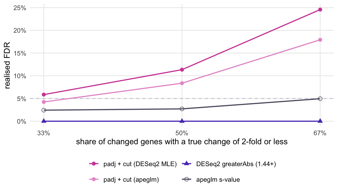
Figure 3: Realised FDR for the size claim with five samples per group, against the share of changed genes whose true change is 2-fold or less, averaged over the simulated datasets. The dashed line is the nominal level.
With two thirds of the changes below 2-fold, the cut’s false share rose to 24.6% (17.9% with apeglm). With one third, it came down to 5.9% (4.2%), close to the nominal level: when fewer genes change by a little, a cut does less harm. DESeq2’s threshold test (the current formula) made no false calls for the size claim in either setting, but with two thirds of the changes below 2-fold it called only 3 genes per dataset on average and found 1.0% of the larger changes, so that result rests on very few calls (see the table). The s-value’s false share also rose with the share of small changes, from 2.4% to 4.9%, which puts it close to the nominal level in the least friendly setting; with a spread of effect sizes that its prior fits worse, it could go above.
So the error of the post hoc cut is not a fixed penalty you could correct for. It grows with the share of genes that changed a little, which is what the experiment was meant to find out.
PyDESeq2 (Muzellec et al. 2023) has a threshold test too. In version 0.5.4, DeseqStats() takes lfc_null, the threshold on the log2 scale, and alt_hypothesis; the script checks that both names exist in the installed version. Its "greaterAbs" p-value, in the package source, is the 2014 formula (twice the one-sided tail), so it matches greaterAbs2014 in current DESeq2, not DESeq2’s current "greaterAbs". Set both: with alt_hypothesis left at its default of None, the Wald test asks whether the fold change equals lfc_null, not whether it is larger in absolute value. The script simulates 3 datasets of 2,500 genes with 5 samples per group the same way as above, with numpy’s random generator, so the draws differ from the R run. The cut after padj gave a false share of 11.9% for the size claim (power 78.8%); the threshold test gave 0.4% (power 17.1%), in line with the greaterAbs2014 row of the R table at 5 samples per group.
# PyDESeq2: a fold-change cut-off after padj versus a test against the threshold.# Simulates negative binomial counts the same way as the R code in the post (with# numpy's random generator, so the datasets are not identical to the R ones), runs# PyDESeq2 once per dataset and scores two ways of calling "more than 2-fold" genes.import csvimport importlib.metadata as mdimport inspectimport numpy as npimport pandas as pdfrom pydeseq2.dds import DeseqDataSetfrom pydeseq2.ds import DeseqStatsn_per, n_genes, n_exp =5, 2500, 3# samples per group, genes per dataset, datasetsp_change, lfc_max =0.4, 2.0# share of genes that change; |true LFC| ~ U(0, lfc_max)threshold, alpha =1.0, 0.05# size claim |log2 FC| > 1; FDR level# the argument names used below, read from the installed versionstats_args = inspect.signature(DeseqStats.__init__).parametersassert"lfc_null"in stats_args and"alt_hypothesis"in stats_argsrng = np.random.default_rng(2026)def simulate(): mu0 = np.exp(rng.normal(np.log(40), 1.6, n_genes)) phi = (0.04+0.2/ np.sqrt(mu0 +1)) * np.exp(rng.normal(0, 0.3, n_genes)) changed = rng.random(n_genes) < p_change lfc = np.where(changed, rng.choice([-1, 1], n_genes) * rng.uniform(0, lfc_max, n_genes), 0) group = np.repeat([0, 1], n_per) sf = np.exp(rng.normal(0, 0.15, 2* n_per)) mu = mu0[:, None] * sf[None, :] *2.0** (lfc[:, None] * group[None, :]) size =1/ phi[:, None] counts = rng.negative_binomial(size, size / (size + mu)) # mean mu, dispersion phireturn counts.T, lfc, groupdef score(call, lfc): big = np.abs(lfc) > threshold n =int(call.sum()) fdp =float(np.mean(~big[call])) if n else0.0return n, fdp, float((call & big).sum() / big.sum())rows = {"post": [], "test": []}for e inrange(n_exp): counts, lfc, group = simulate() genes = [f"g{i}"for i inrange(n_genes)] meta = pd.DataFrame({"condition": np.where(group ==1, "B", "A")}, index=[f"s{i}"for i inrange(2* n_per)]) dds = DeseqDataSet(counts=pd.DataFrame(counts, index=meta.index, columns=genes), metadata=meta, design="~condition", quiet=True, n_cpus=1) dds.deseq2()# the usual route: test against zero, then cut on the estimated fold change st0 = DeseqStats(dds, contrast=["condition", "B", "A"], alpha=alpha, quiet=True, n_cpus=1) st0.summary() r0 = st0.results_df post = ((r0["padj"] < alpha) & (r0["log2FoldChange"].abs() > threshold)).to_numpy()# the test against the threshold: lfc_null is on the log2 scale st1 = DeseqStats(dds, contrast=["condition", "B", "A"], alpha=alpha, quiet=True, n_cpus=1, lfc_null=threshold, alt_hypothesis="greaterAbs") st1.summary() test = (st1.results_df["padj"] < alpha).to_numpy() rows["post"].append(score(post, lfc)) rows["test"].append(score(test, lfc))out = [("n_per_group", n_per), ("n_genes", n_genes), ("n_datasets", n_exp)]for k, v in rows.items(): a = np.array(v) out += [(f"calls_{k}", a[:, 0].mean()), (f"fdr_{k}", a[:, 1].mean()), (f"fdr_{k}_max", a[:, 1].max()), (f"power_{k}", a[:, 2].mean())]out += [("pydeseq2_version", md.version("pydeseq2")), ("numpy_version", md.version("numpy"))]withopen("lfc_threshold_check-results.csv", "w", newline="") as f: w = csv.writer(f) w.writerow(["name", "value"]) w.writerows(out)
What to do in practice
Decide before looking at the results whether the size of the change is part of your claim.
If it is, put the threshold into the test and state the threshold with the list. The edgeR and limma authors’ advice is to use a modest threshold, such as log2(1.2) or log2(1.5), and make the claim at that size (“changed by more than 1.5-fold”); sorting that list by fold change is fine, as long as a 2-fold subset is described as a ranking choice, not a result. If the claim has to be “more than 2-fold”, test at 1 and expect a short list, longer with more samples. In DESeq2, name the altHypothesis and the DESeq2 version in your methods, since "greaterAbs" changed in 1.44.
If the size is not part of your claim, test against zero and report the genes at your FDR. You can still sort or filter that list by fold change for follow-up, but say that the fold-change filter is a choice of which genes to look at, not a second statistical result.
# DESeq2: genes whose absolute log2 fold change is greater than 1, at 5% FDR# ("greaterAbs" is the newer formula from DESeq2 1.44; "greaterAbs2014" gives the old one)res_thr <-results(dds, lfcThreshold =1, altHypothesis ="greaterAbs", alpha =0.05)summary(res_thr)# DESeq2 + apeglm: shrunken estimates and s-values for the same claimres_ape <-lfcShrink(dds, coef =2, type ="apeglm", lfcThreshold =1)subset(res_ape, svalue <0.05)# edgeR: quasi-likelihood fit, then a test against a modest threshold (claim: > 1.5-fold)keep <-filterByExpr(y, group = group)y <-normLibSizes(y[keep, , keep.lib.sizes =FALSE])fit <-glmQLFit(y, design, robust =TRUE, legacy =FALSE)tr <-glmTreat(fit, coef =2, lfc =log2(1.5)) # lfc = 1 for a 2-fold claimtopTags(tr, p.value =0.05, n =nrow(y))# limma-voom, same claimv <-voom(y, design)fit_l <-lmFit(v, design)topTreat(treat(fit_l, lfc =log2(1.5)), coef =2, p.value =0.05, number =nrow(v))
Three smaller points. In this simulation edgeR’s filterByExpr() removed 19% of genes before testing, and those count as missed in the power column of the table below; DESeq2 filters differently, inside results(). And the threshold tests inherit the usual limits of the underlying test, so a gene with very few reads and an extreme estimate can still pass them; expression filtering matters as much as before. Finally, a threshold test changes the p-value histogram. With DESeq2’s 2014 formula every gene whose estimate lies inside the threshold gets a p-value of exactly 1 (78% of genes here); with the current formula they all get a p-value of at least 0.5, since the tail beyond the nearer boundary alone is at least a half. The shapes described in the post on p-value histograms are for tests against zero and do not apply to either.
All the analyses side by side, averaged over the 4 datasets per sample size: