Independent filtering: when gene filters break the FDR
DESeq2
edgeR
FDR
RNA-seq
multiple testing
Can you filter genes before multiple testing correction? Independent filtering on mean count keeps the FDR and adds power; a fold-change pre-filter breaks it.
Author
Pseudocount
Published
11 September 2026
Setup: packages and helper functions
suppressPackageStartupMessages({library(DESeq2)library(edgeR)library(ggplot2)})stopifnot(packageVersion("DESeq2") >="1.36", packageVersion("edgeR") >="4.0.0",packageVersion("ggplot2") >="3.4.0")pct <-function(x, d =1) sprintf(paste0("%.", d, "f%%"), 100* x)num <-function(x) format(round(x), big.mark =",", scientific =FALSE, trim =TRUE)dec <-function(x, d =2) sprintf(paste0("%.", d, "f"), x)fdr_level <-0.05# genes are called at this Benjamini-Hochberg adjusted p-value# Benjamini-Hochberg on the genes in `keep` only; the rest stay missingbh_on <-function(p, keep) { padj <-rep(NA_real_, length(p)) ok <- keep &!is.na(p) padj[ok] <-p.adjust(p[ok], "BH") padj}# what we can measure because the truth is knownscore <-function(padj, is_de) { call <-!is.na(padj) & padj < fdr_levelc(n_call =sum(call),fdp =if (any(call)) mean(!is_de[call]) else0, # false discovery proportionpower =sum(call & is_de) /sum(is_de)) # share of ALL changed genes found}# the defaults this post talks about, read from the installed packagesresults_alpha <-eval(formals(DESeq2::results)$alpha)results_indep <-eval(formals(DESeq2::results)$independentFiltering)results_althyp <-eval(formals(DESeq2::results)$altHypothesis)[1]fbe_min_count <-eval(formals(edgeR:::filterByExpr.default)$min.count)fbe_min_total <-eval(formals(edgeR:::filterByExpr.default)$min.total.count)
You have a results table with a few thousand genes, many of them barely expressed, and you would like to drop the uninteresting ones before correcting for multiple testing. Is that allowed? Yes, if the filter ignores which sample is in which group and is (approximately) independent of the test for genes that do not change, as the mean count is; no, if it looks at the groups. In the simulation below, filtering on expression kept the realised false discovery rate (FDR) at 4.7% with edgeR and 4.7% with DESeq2’s automatic filter, for a nominal 5%, and DESeq2’s filter called 6.0% more genes than no filter at all. Keeping only genes with at least a 1.4-fold difference between the groups before the correction pushed the realised FDR to 16.4%.
Why removing genes can add power
The usual FDR correction is the Benjamini-Hochberg procedure (Benjamini and Hochberg 1995). It sorts the p-values of all tested genes and compares the k-th smallest with k/m times the target FDR, where m is the number of genes tested. The larger m is, the higher the bar every gene has to clear. In RNA-seq a large share of genes have so few reads that they could never produce a small p-value, whatever their true change, yet each of them adds to m. Removing them before the correction lowers the bar for the rest. (The same genes bend the p-value histogram towards 1, as shown in the post on p-value histograms; here the question is what removing them does to the FDR.)
The catch is in how you choose which genes to remove. The procedure’s guarantee rests on the p-values of null genes, genes with no true change, being spread evenly between 0 and 1. Bourgon, Gentleman and Huber (2010) showed that filtering keeps this property when, for null genes, the filter statistic is independent of the test statistic. The overall mean count, computed across all samples without looking at the group labels, is the standard example. A statistic that looks at the difference between the groups is not: a null gene whose groups differ by chance has both a large difference and a small p-value, so a filter on the difference hands the correction a set of null genes with too many small p-values. The simulation below measures both.
The setup
Each simulated experiment has 3,000 genes measured in 4 control and 4 treated samples, with counts drawn from a negative binomial distribution (the standard model for RNA-seq counts, in which the variance grows faster than the mean). Mean counts are spread over several orders of magnitude, so that 49% of genes average fewer than 10 reads per sample, much as in a real annotation with many barely expressed genes. The dispersion, the biological part of the variance, is larger for weakly expressed genes. In each experiment 15% of genes truly change, with a log2 fold change between 0.5 and 2 in either direction; the rest are null.
I simulate 16 experiments and report averages over them, because the FDR is itself an average over experiments: in a single experiment the share of false calls can land above the target without anything being wrong.
Two assumptions deserve a flag. Genes are simulated independently of each other, while real genes are correlated. And the share of changed genes and the size of their changes are my choices; the last section shows that the damage done by a bad filter depends on the first.
DESeq2 runs its standard workflow, DESeq() then results() (Love, Huber and Anders 2014). To save time it is run once on all experiments stacked on top of each other; they share the 8 samples’ sequencing depths and the fitted dispersion trend, and every experiment is filtered, corrected and scored on its own. edgeR runs per experiment with the quasi-likelihood recipe of Chen, Lun and Smyth (2016), updated with the current filterByExpr() and normLibSizes(): filter, normalise, then glmQLFit() and glmQLFTest(). The fit uses edgeR’s newer quasi-likelihood method, legacy = FALSE, set explicitly so that older and newer edgeR releases run the same method; this method estimates its own dispersion, so estimateDisp() is not needed.
# one DESeq2 fit for all experiments (to save time); each experiment is scored on its own belowdds <-DESeqDataSetFromMatrix(sim$counts, data.frame(group = group), ~ group)dds <-DESeq(dds, quiet =TRUE)res_all <-results(dds, independentFiltering =FALSE)low_count <-10share_low <-mean(res_all$baseMean < low_count)# the edgeR quasi-likelihood recipe, filterByExpr firstrun_edger <-function(counts, fc_cut) { y <-DGEList(counts, group = group) keep <-filterByExpr(y, group = group) y <-normLibSizes(y[keep, , keep.lib.sizes =FALSE]) fit <-glmQLFit(y, design, robust =TRUE, legacy =FALSE) tab <-glmQLFTest(fit, coef =2)$table treat <-glmTreat(fit, coef =2, lfc = fc_cut)$table # used in the last section p <- lfc <- p_treat <-rep(NA_real_, nrow(counts)) p[keep] <- tab$PValue; lfc[keep] <- tab$logFC; p_treat[keep] <- treat$PValuelist(p = p, lfc = lfc, keep = keep, p_treat = p_treat)}
The next chunk scores every analysis in this post on each experiment: DESeq2 with and without its automatic filter, the edgeR recipe, both with a fold-change pre-filter added, and the two threshold tests from the last section.
fc_cut <-0.5# |log2 fold change| cut-off of the pre-filterthresholds <-c(0, 0.25, 0.5, 0.75, 1, 1.5) # cut-offs for the sweep further downper_exp <-lapply(seq_len(n_exp), function(e) { i <-which(experiment == e) de <- sim$is_de[i] p <- res_all$pvalue[i] fc <-abs(res_all$log2FoldChange[i]) auto <-results(dds[i, ], alpha = fdr_level) # automatic independent filtering auto_default <-results(dds[i, ]) # same, alpha left at its default treat <-results(dds[i, ], lfcThreshold = fc_cut, alpha = fdr_level) ed <-run_edger(sim$counts[i, ], fc_cut) fc_keep <-!is.na(fc) & fc > fc_cut below_cut <- res_all$baseMean[i] <metadata(auto)$filterThreshold ed_fc_keep <- ed$keep &abs(ed$lfc) > fc_cut ed_padj <-bh_on(ed$p, ed$keep) # correction first ... post_cut <-function(cut) ifelse(abs(ed$lfc) > cut, ed_padj, NA_real_) # ... then a fold-change cutlist(rows =rbind(deseq_none =score(bh_on(p, TRUE), de),deseq_auto =score(auto$padj, de),deseq_fc =score(bh_on(p, fc_keep), de),edger =score(bh_on(ed$p, ed$keep), de),edger_fc =score(bh_on(ed$p, ed_fc_keep), de),deseq_treat =score(treat$padj, de),edger_treat =score(bh_on(ed$p_treat, ed$keep), de)),auto_default =score(auto_default$padj, de),post =rbind(small =score(post_cut(fc_cut), de), large =score(post_cut(1), de)),null_share_fc =mean(!de[ed_fc_keep]),filtered =mean(is.na(auto$padj)),sweep =sapply(thresholds, function(t) c(deseq =score(bh_on(p, !is.na(fc) & fc > t), de)[["fdp"]],edger =score(bh_on(ed$p, ed$keep &abs(ed$lfc) > t), de)[["fdp"]])),# null p-values that survive each filter, for the histogramnull_p =rbind(data.frame(p = ed$p[ed$keep &!de], filter ="recipe"),data.frame(p = ed$p[ed_fc_keep &!de], filter ="fold"),data.frame(p = p[fc_keep &!de],filter =ifelse(below_cut[fc_keep &!de], "deseq_fold_low", "deseq_fold_high"))),auto =if (e ==1) auto elseNULL)})tab <-Reduce(`+`, lapply(per_exp, `[[`, "rows")) / n_expauto_default <-colMeans(do.call(rbind, lapply(per_exp, `[[`, "auto_default")))filtered_share <-mean(sapply(per_exp, `[[`, "filtered"))gain <- tab["deseq_auto", "n_call"] / tab["deseq_none", "n_call"] -1fdp_fc_edger <-sapply(per_exp, function(x) x$rows["edger_fc", "fdp"])fdp_recipe <-sapply(per_exp, function(x) x$rows["edger", "fdp"])n_fc_worse <-sum(fdp_fc_edger > fdp_recipe)null_p <-do.call(rbind, lapply(per_exp, `[[`, "null_p"))null_sig <-tapply(null_p$p < fdr_level, null_p$filter, mean)deseq_null <- null_p[null_p$filter %in%c("deseq_fold_low", "deseq_fold_high"), ]deseq_null_sig <-mean(deseq_null$p < fdr_level)deseq_fc_null_low <-mean(deseq_null$filter =="deseq_fold_low")sweep <-Reduce(`+`, lapply(per_exp, `[[`, "sweep")) / n_expnull_share_fc <-mean(sapply(per_exp, `[[`, "null_share_fc"))post <-Reduce(`+`, lapply(per_exp, `[[`, "post")) / n_expauto1 <- per_exp[[1]]$auto
Filtering on expression
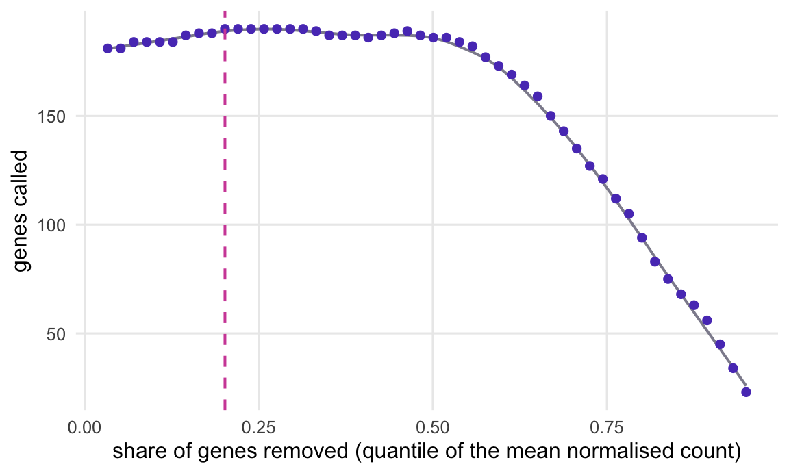
DESeq2 filters for you. With the default independentFiltering = TRUE, results() filters on the mean of normalised counts across all samples. It tries a series of cut-offs, counts the genes called at each, and keeps the lowest cut-off whose count comes within one residual standard deviation of the peak of a curve fitted through those counts (this is described in the DESeq2 vignette). Genes below the cut-off keep their p-value, but their adjusted p-value is left empty. The search for the first experiment looks like this:
nr <-metadata(auto1)$filterNumRejlo <-as.data.frame(metadata(auto1)$lo.fit)ggplot(nr, aes(theta, numRej)) +geom_line(data = lo, aes(x, y), colour ="#8e8c9c", linewidth =0.7) +geom_point(colour ="#5a3fc0", size =1.8) +geom_vline(xintercept =metadata(auto1)$filterTheta, linetype ="dashed",colour ="#d14fa6", linewidth =0.7) +labs(x ="share of genes removed (quantile of the mean normalised count)",y ="genes called") +theme_minimal(base_size =12) +theme(panel.grid.minor =element_blank(),plot.background =element_rect(fill ="white", colour ="white"))
Figure 1: DESeq2’s search for an independent filtering cut-off in the first simulated experiment. Each point is the number of genes called after removing the given share of genes with the lowest mean count; the grey line is the fitted curve and the dashed line marks the chosen cut-off.
In this experiment the chosen cut-off removes the 20% of genes whose mean normalised count is below 1.26. Across all experiments it removed 26% of genes on average. DESeq2 then called 172 genes per experiment against 163 without the filter, and found 36.5% of the truly changed genes instead of 34.9%. The realised FDR was 4.7% with the filter and 3.5% without it, both below the nominal level. The gain is modest in this simulation; how large it is in your data depends on how many genes in the table have too few reads to ever be significant.
One detail matters here. The cut-off is chosen to maximise the calls at the significance level alpha, whose default is 0.1. If you call genes at an adjusted p-value of 0.05, the vignette says to set alpha to that value too. Leaving it at the default made little difference in this simulation (171 against 172 genes called), but it costs nothing to set.
edgeR filters before the model is fitted. filterByExpr() keeps genes with at least min.count reads (default 10, converted to counts per million with the median library size) in at least as many samples as the smallest group, and at least min.total.count reads in total (default 15). It uses the group sizes only to decide how many samples a gene must be expressed in; it counts those samples across all columns, so the result does not depend on which sample sits in which group. With filterByExpr() first, the edgeR recipe had a realised FDR of 4.7% and found 35.5% of the changed genes.
Filtering on a fold change
Now the tempting shortcut: keep only genes whose groups differ by at least 1.4-fold (an absolute log2 fold change above 0.5), taken from the same results table, and run the correction on those. Added to the edgeR recipe, this raised the calls from 167 to 223 per experiment and the realised FDR from 4.7% to 16.4%. The false discovery proportion was higher with the fold-change filter in every one of the 16 experiments, ranging from 12.0% to 21.1%.
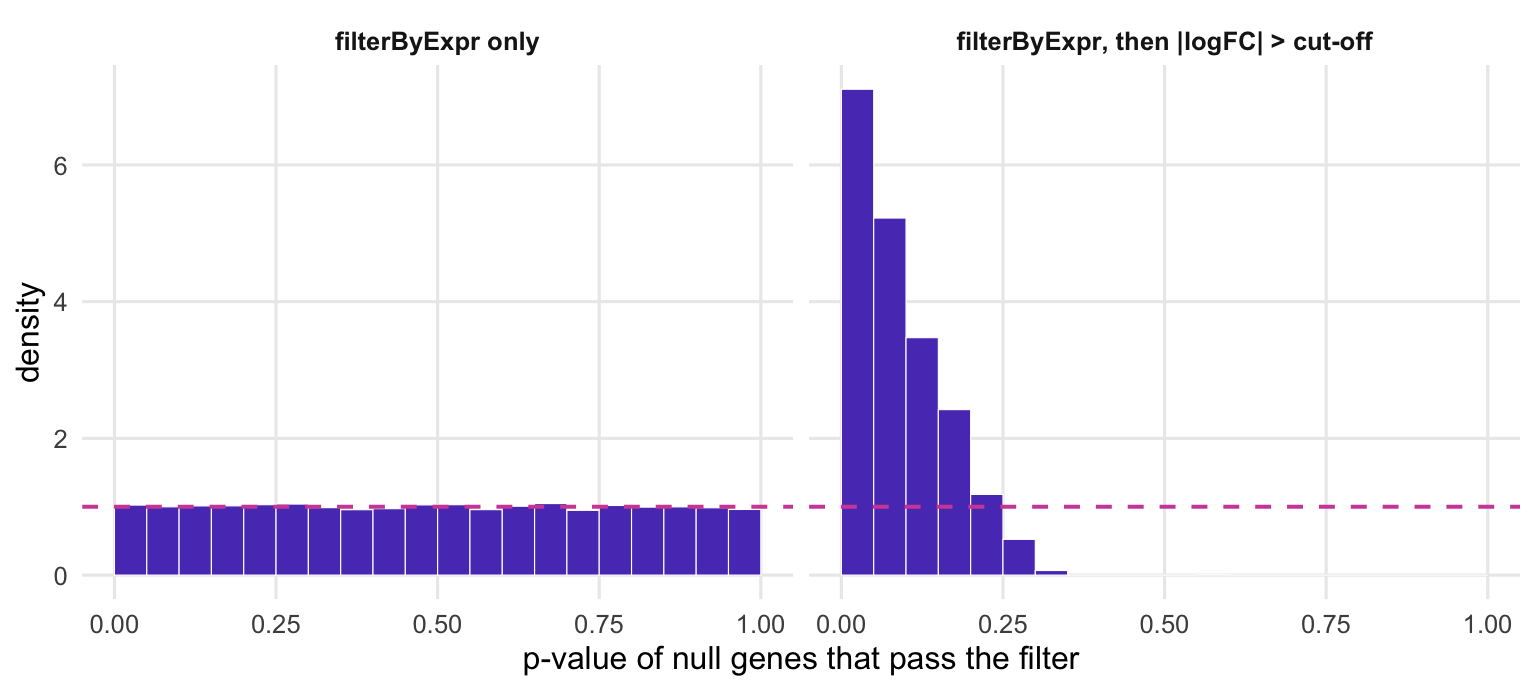
The reason is visible in the null genes that survive the filter.
Figure 2: P-values of null genes that pass each filter, pooled over the simulated experiments, from the edgeR recipe. After filterByExpr alone they are spread evenly (left); after an added fold-change filter they pile up near zero (right). The dashed line is the flat density that null p-values should have.
Among null genes that pass filterByExpr(), 5.1% have a p-value below 0.05, which is what a p-value promises. Among null genes that also pass the fold-change filter, 35.5% do. The correction receives a set of genes with far more small p-values than its null model allows for, and treats the excess as signal.
The same filter on DESeq2’s p-values, applied to all genes, raised the realised FDR from 3.5% to 7.1%. That is a smaller rise, and the reason says something about the mechanism. DESeq2’s fold change for a gene with a handful of reads is very noisy, so many null genes with almost no reads pass a fold-change filter: 48% of the null genes that passed had a mean count below the automatic filter’s cut-off. Only 0.8% of those had a p-value below 0.05, against 16.5% of the better expressed null genes that passed, so the low-count genes dilute the problem without removing it. Overall, 8.9% of the null genes passing this filter had a p-value below 0.05, still more than a p-value promises.
The damage depends on what you cannot see
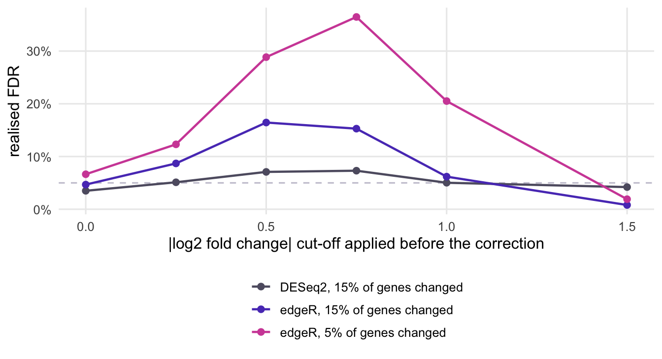
Is a larger cut-off safer? The next figure repeats the fold-change filter at several cut-offs and adds a second scenario, simulated the same way except that only 5% of genes truly change.
de_frac_low <-0.05# a second scenario: fewer genes truly changeset.seed(2027)sim_low <-simulate(n_genes * n_exp, de_frac_low, n_genes)null_share_fc_low <-numeric(n_exp)fdp_low <-sapply(seq_len(n_exp), function(e) { i <-which(experiment == e) ed <-run_edger(sim_low$counts[i, ], fc_cut) null_share_fc_low[e] <<-mean(!sim_low$is_de[i][ed$keep &abs(ed$lfc) > fc_cut])sapply(thresholds, function(t)score(bh_on(ed$p, ed$keep &abs(ed$lfc) > t), sim_low$is_de[i])[["fdp"]])})sweep_low <-rowMeans(fdp_low)se_low <-apply(fdp_low, 1, sd) /sqrt(n_exp) # Monte Carlo standard error
Figure 3: Realised FDR after a fold-change pre-filter, against the cut-off, averaged over the simulated experiments. The dashed line is the nominal level. The filter pushes the FDR above it over a range of cut-offs, and by how much depends on the share of genes that truly change.
With no cut-off the analyses sit near the nominal level. The edgeR run in the second scenario is slightly above it, at 6.6% with a Monte Carlo standard error of 0.7% (the uncertainty that comes from simulating only 16 experiments). Any cut-off in the middle of the range pushes the FDR up, and the push is larger when fewer genes truly change, because a larger share of what passes the filter is then null: at a cut-off of 0.5, 73% of the genes passing were null in the second scenario against 46% in the first. In the second scenario the realised FDR peaked at 36.5% at a cut-off of 0.75. At the popular two-fold cut-off (log2 fold change 1), edgeR’s realised FDR was 6.2% in the first scenario and 20.5% in the second. At the largest cut-off, 1.5, it falls to 1.9%.
So the harm from a fold-change pre-filter is not a fixed penalty you could correct for. It depends on how many genes truly change (and, by the same logic, on how large the changes are), which is exactly what the experiment is trying to find out. A cut-off that looks harmless on one data set carries no guarantee on the next.
What to do in practice
Filter on expression, and never on anything that uses the group labels. Ignoring the labels is necessary but not sufficient: Bourgon, Gentleman and Huber (2010) show that some filter and test pairs lose control of false positives even so, so stay with the filters the packages provide, which were checked here: the mean count in DESeq2 and filterByExpr() in edgeR. In DESeq2 that means leaving the automatic filter on and setting alpha to the adjusted p-value cut-off you will use. In edgeR it means running filterByExpr() before fitting.
If you only care about changes above a certain size, put the size into the test rather than into a filter. DESeq2’s results() takes lfcThreshold; with the default altHypothesis = "greaterAbs" it tests whether the absolute log2 fold change is greater than the threshold. edgeR’s glmTreat() does the same for a fitted quasi-likelihood model, based on the TREAT approach of McCarthy and Smyth (2009). Its help page adds a warning: the threshold in the test is not a fold-change cut-off, because a gene needs an observed change well above it to be called, so modest thresholds such as log2(1.2) or log2(1.5) are usually the most useful.
These tests answer a stricter question, so they call fewer genes. With a threshold of 0.5, DESeq2 called 91 genes per experiment and edgeR 123, with realised FDRs of 0.1% and 0.8%. (A call counts as false when the gene did not change at all; no gene in this simulation has a true change between zero and the threshold.)
A fold-change cut applied after the correction, as in the common padj < 0.05 plus a minimum fold change, is a different thing. It only removes genes from a list whose FDR is already controlled. In the edgeR runs, cutting the called genes at an absolute log2 fold change of 0.5 removed none of them, since every called gene already had a larger observed change, with a realised FDR of 4.7%, and a cut at 1 left 148 genes with 2.6%. It did not raise the FDR here, but it is not a test of the size of the change either: nothing guarantees that a gene which passes has a true change above the cut-off. When the size matters, use lfcThreshold or glmTreat().
# DESeq2: automatic independent filtering, tuned to the cut-off you will useres <-results(dds, alpha =0.05)metadata(res)$filterThreshold # the mean-count cut-off it chosesummary(res)# DESeq2: only changes larger than about 1.4-fold, tested rather than filteredres_big <-results(dds, lfcThreshold =0.5, alpha =0.05)# edgeR: filter on expression before fittingkeep <-filterByExpr(y, group = group)y <-normLibSizes(y[keep, , keep.lib.sizes =FALSE])fit <-glmQLFit(y, design, robust =TRUE, legacy =FALSE)qlf <-glmQLFTest(fit, coef =2) # any changetr <-glmTreat(fit, coef =2, lfc =log2(1.5)) # changes above a thresholdtopTags(tr)
All the analyses side by side, averaged over the 16 experiments: