Comparing cell type proportions in single-cell data
scRNA-seq
compositional data
edgeR
limma
How to compare cell type proportions between conditions in single-cell data: a simulation of pooled chi-square and cell shuffling against propeller and edgeR.
You have clustered single-cell data from treated and control donors, and one cluster looks larger in the treated cells. The question people then type into a search box is how to compare cell type proportions between conditions, and a common answer is to add up the cells of each condition and run a chi-square or Fisher test per cluster, or a permutation test that shuffles the condition labels between cells.
These tests treat every cell as an independent observation, and when donors differ in composition they report changes that are not there. In the simulation below, with 3 donors per condition and no true change in any cluster, the pooled chi-square test gave p < 0.05 in 81% of cluster comparisons. Two tests that use the donor as the replicate, the transformation propeller uses followed by limma, and edgeR on cluster counts, gave 6.2% and 6.2% (nominal 5%).
The setup
base_prop <-c(C1 =0.30, C2 =0.20, C3 =0.15, C4 =0.10,C5 =0.08, C6 =0.07, C7 =0.06, C8 =0.04)# one donor x cluster table of cell countssimulate_table <-function(n_per_group, conc =100, fold =1, target ="C2",cells =c(2000, 10000)) { n <-2* n_per_group group <-factor(rep(c("ctrl", "trt"), each = n_per_group)) total <-round(runif(n, cells[1], cells[2])) # cells captured per donor counts <-t(vapply(seq_len(n), function(i) { p <- base_propif (group[i] =="trt") { # optional true change p[target] <- p[target] * fold p <- p /sum(p) }if (!is.null(conc)) { # Dirichlet: donor's own composition g <-rgamma(length(p), shape = p * conc) p <- g /sum(g) }rmultinom(1, total[i], p)[, 1] # cells sampled from that donor }, numeric(length(base_prop))))dimnames(counts) <-list(sprintf("d%02d", seq_len(n)), names(base_prop))list(counts = counts, group = group)}conc_main <-formals(simulate_table)$conccell_range <-eval(formals(simulate_table)$cells)sd_prop <-sqrt(base_prop * (1- base_prop) / (conc_main +1)) # Dirichlet sd per clustercv_prop <- sd_prop / base_propn_clust <-length(base_prop)n_per_group <-3# the example below
Only the table of cell counts per donor and cluster is simulated, because that table is all any of these tests uses. There are 8 clusters with baseline shares from 30% (C1) down to 4% (C8). Each donor gets its own composition, drawn from a Dirichlet distribution centred on the baseline, and then between 2,000 and 10,000 cells are sampled from that composition (a multinomial draw). Both conditions share the same baseline, so no cluster truly changes.
How much donors differ is the assumption that matters. The Dirichlet concentration of 100 gives a standard deviation between donors of 4.6 percentage points for C1 and 1.9 for C8, or 15% and 49% of their baseline shares: rare clusters vary more, relative to their size. Real donors can differ more or less than this, depending on the tissue, the individuals and how reproducible the dissociation is, so a later section varies it down to no donor variation at all.
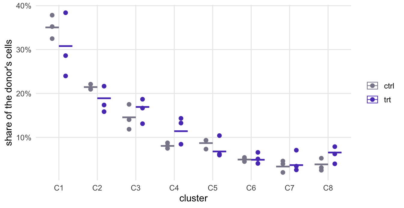
The table below and Figure 1 show one simulated experiment with 3 donors per condition.
Figure 1: One simulated experiment with no true condition effect. Each point is one donor’s proportion of cells in a cluster; the bars are the proportions after pooling all cells of a condition.
The common way: cells as the unit
# cells summed per condition, then one 2 x 2 test per cluster: this cluster vs the restpooled_tests <-function(counts, group) { s <-rowsum(counts, group) total <-rowSums(s)t(vapply(colnames(counts), function(k) { tab <-cbind(s[, k], total - s[, k])c(chisq =chisq.test(tab)$p.value, fisher =fisher.test(tab)$p.value) }, numeric(2)))}p_pooled_ex <-pooled_tests(ex$counts, ex$group)
# cell shuffling: give every cell its condition, shuffle the labels across cells,# and compare the observed difference in proportion with the shuffled onesshuffle_test <-function(counts, group, B =999) { cluster <-rep(rep(seq_len(ncol(counts)), nrow(counts)), as.vector(t(counts))) n_trt <-sum(counts[group =="trt", ]) N <-length(cluster) diff_prop <-function(in_trt) { k_trt <-tabulate(cluster[in_trt], ncol(counts)) k_trt / n_trt - (tabulate(cluster, ncol(counts)) - k_trt) / (N - n_trt) } obs <-diff_prop(rep(group, rowSums(counts)) =="trt") perm <-replicate(B, diff_prop(sample.int(N, n_trt)))setNames((1+rowSums(abs(perm) >=abs(obs))) / (B +1), colnames(counts))}set.seed(2)p_shuffle_ex <-shuffle_test(ex$counts, ex$group)
The common analysis sums the cells of each condition and asks, cluster by cluster, whether the share of cells in that cluster differs between the two pooled groups: a 2 x 2 table (in this cluster or not, control or treated) tested with chisq.test() or fisher.test(). On this one experiment, with 37,750 cells in total, the chi-square test gives p < 0.05 for 6 of the 8 clusters, although none changed. Fisher’s test gives nearly the same p-values (largest difference 0.010).
Cell shuffling is the permutation version of the same idea, and a common answer on Q&A forums. It gives every cell its donor’s condition, shuffles those labels across cells, and compares the observed difference in a cluster’s share with the shuffled differences. With 999 shuffles the smallest possible p-value is 0.001, and 6 clusters fall below 0.05.
Both tests answer this question: if every cell were an independent draw from one set of proportions shared by both conditions, how surprising would the table be? That hypothesis is false here even though the conditions do not differ, because the cells of a donor share that donor’s composition. With thousands of cells per condition, the donor-to-donor differences in Figure 1 are far larger than the sampling noise the test allows for, so it reports them as evidence. Shuffling cells does not repair this, since it breaks the donors up: the null distribution it builds contains no donor variation. The same mistake in differential expression, cells treated as replicates, is the subject of the pseudobulk post.
Testing at the donor level
# the transformation propeller uses (Phipson et al. 2022), then limma as propeller runs itpropeller_like <-function(counts, group, transform =c("logit", "asin")) { transform <-match.arg(transform)if (transform =="logit") { p <- (counts +0.5) /rowSums(counts +0.5) # 0.5 added to every count y <-t(log(p / (1- p))) } else { y <-t(asin(sqrt(counts /rowSums(counts)))) } design <-model.matrix(~0+ group) # one column per condition fit <-contrasts.fit(lmFit(y, design), c(-1, 1)) # trt minus ctrleBayes(fit, robust =TRUE)$p.value[, 1]}# edgeR quasi-likelihood on cluster counts, library size = cells per donor (OSCA recipe)edger_da <-function(counts, group, tmm =FALSE) { y <-DGEList(t(counts), group = group) keep <-filterByExpr(y, group = group) y <- y[keep, , keep.lib.sizes =FALSE]if (tmm) y <-normLibSizes(y) # only for the composition fix below design <-model.matrix(~ group) y <-estimateDisp(y, design, trend.method ="none") fit <-glmQLFit(y, design, dispersion = y$common.dispersion, robust =TRUE,abundance.trend =FALSE, legacy =FALSE) p <-setNames(rep(NA_real_, ncol(counts)), colnames(counts)) p[rownames(y)] <-glmQLFTest(fit, coef =2)$table$PValue p}p_donor_ex <-cbind(propeller_logit =propeller_like(ex$counts, ex$group),edgeR_QL =edger_da(ex$counts, ex$group))
The experiment has 6 donors, and the donor is the replicate. Two tests use it.
propeller (Phipson et al. 2022), in the Bioconductor package speckle, turns each donor’s counts into proportions, transforms them, and fits a linear model per cluster with limma, whose empirical Bayes step borrows information about variability across clusters. propeller_like() above follows the propeller code in speckle (read in the Bioconductor 3.18 branch; the three functions involved are unchanged in the 3.22 branch): for the default logit transformation it adds 0.5 to every count before computing proportions, the design has one column per condition, and eBayes() runs with robust = TRUE (limma’s own default is FALSE). Run on the same tables, it returns the same p-values as speckle::propeller(); speckle is not loaded here so that the page runs without it.
The second test is the recipe in the differential abundance chapter of the Orchestrating Single-Cell Analysis book, which follows an approach first used for mass cytometry (Lun et al. 2017): treat the cluster counts of each donor like gene counts in bulk RNA-seq, with the donor’s total number of cells as the library size, and run edgeR’s quasi-likelihood test. The book skips calcNormFactors() on purpose, so that the test is about proportions; it estimates the negative binomial dispersion with estimateDisp(..., trend = "none") and fits glmQLFit() with robust = TRUE and abundance.trend = FALSE, because a handful of clusters cannot support a trend. Two settings are added here. legacy = FALSE selects the quasi-likelihood method of edgeR 4 (the default changed between versions, so it is set explicitly); details of its estimation changed between edgeR 4.0 and 4.8, so edgeR numbers from a newer installation differ slightly from the ones on this page. The second setting is the dispersion. Without one, glmQLFit(legacy = FALSE) estimates the negative binomial dispersion from the most abundant rows: in edgeR 4.0 (Bioconductor 3.18) the top 5%, which in a table of eight clusters is a single cluster. edgeR 4.8 chooses the proportion from the number of rows and the residual degrees of freedom, and for a table this small uses all or nearly all clusters. On the example table, with the edgeR 4.8.2 that produced this page, glmQLFit() left to itself estimates a dispersion of 0.066, against 0.066 from estimateDisp(). The code therefore passes the common dispersion from estimateDisp(). The edgeR 4.8 help page warns against presetting the dispersion without a reason; the reason here is that the preset value is close to what edgeR 4.8 estimates by itself, while edgeR 4.0, left alone, estimates practically zero.
On the example, both tests give p < 0.05 for 1 cluster (C8). With 8 clusters tested, 0.4 such calls are expected by chance on average; after Benjamini-Hochberg adjustment across clusters (propeller reports it as FDR), the smallest adjusted p-value is 0.24.
False positives over many experiments
# the permutation null of cell shuffling, drawn directly: shuffling the labels of# cells puts a hypergeometric number of each cluster's cells in the treated groupshuffle_fast <-function(counts, group, B =999) { s <-rowsum(counts, group); n <-rowSums(s); kt <-colSums(s)vapply(colnames(counts), function(k) { obs <- s["trt", k] / n["trt"] - s["ctrl", k] / n["ctrl"] x <-rhyper(B, kt[k], sum(n) - kt[k], n["trt"]) perm <- x / n["trt"] - (kt[k] - x) / n["ctrl"] (1+sum(abs(perm) >=abs(obs))) / (B +1) }, numeric(1))}chisq_only <-function(counts, group) { s <-rowsum(counts, group); total <-rowSums(s)vapply(colnames(counts), function(k)chisq.test(cbind(s[, k], total - s[, k]))$p.value, numeric(1))}run_tests <-function(tb) {cbind(chisq =chisq_only(tb$counts, tb$group),shuffle =shuffle_fast(tb$counts, tb$group),propeller_logit =propeller_like(tb$counts, tb$group),propeller_asin =propeller_like(tb$counts, tb$group, "asin"),edgeR_QL =edger_da(tb$counts, tb$group))}n_rep <-500# replicate tables per designdesigns <-c(3, 6) # donors per conditionset.seed(3)null_p <-lapply(designs, function(npg)replicate(n_rep, run_tests(simulate_table(npg)))) # cluster x method x replicatenames(null_p) <- designsfpr <-do.call(rbind, lapply(names(null_p), function(d) { r <-apply(null_p[[d]] < alpha, c(1, 2), mean) # per cluster and methoddata.frame(design =paste(d, "vs", d), method =rep(colnames(r), each =nrow(r)),cluster =rownames(r), fpr =as.vector(r))}))fpr_tab <-aggregate(fpr ~ method + design, fpr, function(v) c(mean =mean(v), min =min(v), max =max(v)))fpr_tab <-do.call(data.frame, fpr_tab)
fpr_tab
            method design fpr.mean fpr.min fpr.max
1            chisq 3 vs 3  0.80875   0.772   0.828
2         edgeR_QL 3 vs 3  0.06225   0.002   0.176
3   propeller_asin 3 vs 3  0.06025   0.044   0.082
4  propeller_logit 3 vs 3  0.06200   0.016   0.164
5          shuffle 3 vs 3  0.80975   0.772   0.830
6            chisq 6 vs 6  0.80700   0.780   0.816
7         edgeR_QL 6 vs 6  0.05900   0.014   0.090
8   propeller_asin 6 vs 6  0.05575   0.026   0.074
9  propeller_logit 6 vs 6  0.05750   0.020   0.082
10         shuffle 6 vs 6  0.80650   0.782   0.818
One experiment shows little either way, so the chunk above repeats the comparison on 500 simulated experiments for each design, 3 vs 3 and 6 vs 6 donors, with no true change anywhere, and records how often each test gives p < 0.05 for each cluster. To save time, the sweep draws the cell-shuffling null directly from the hypergeometric distribution, which is the distribution that shuffling labels across cells produces for one cluster’s count in the treated group.
The table gives the rate averaged over clusters, with the lowest and highest cluster. The pooled chi-square test and cell shuffling call a change in 81% and 81% of null comparisons with 3 donors per condition, and 81% and 81% with 6. More donors do not help them, because their problem is that they ignore donors. The donor-level tests are between 6.0% and 6.2% with 3 donors per condition, a little above the nominal 5%, and between 5.6% and 5.9% with 6.
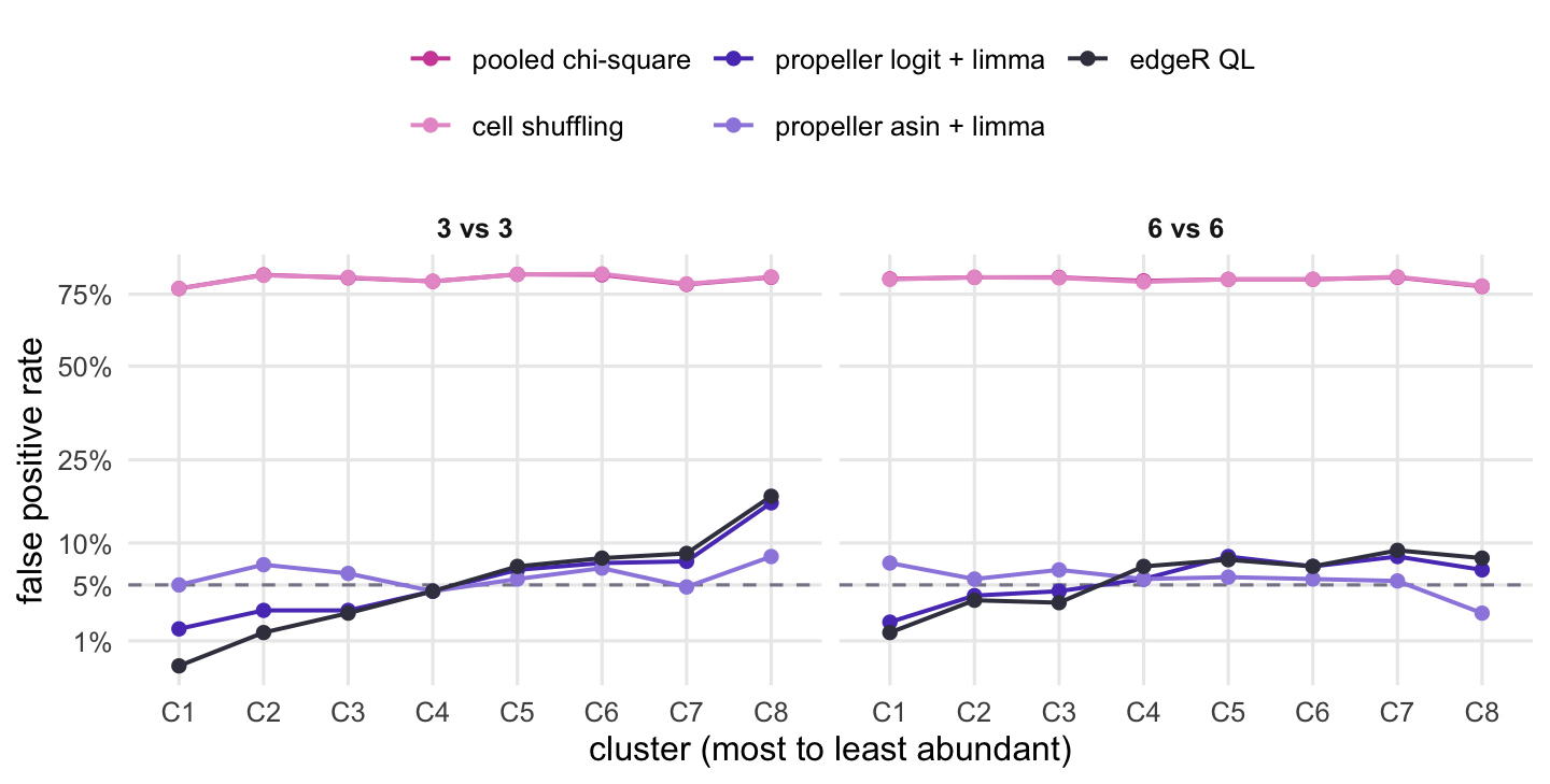
Figure 2 shows the clusters one by one. With 3 donors per condition, the logit version and edgeR are conservative for the most abundant cluster (1.6% and 0.2% for C1) and liberal for the rarest (16.4% and 17.6% for C8), while the arcsine square root version stays between 4.4% and 8.2%. This follows from the simulation. Under a Dirichlet, a rare cluster’s share varies more on the logit scale than an abundant one’s, while the empirical Bayes step pulls every cluster’s variance towards a common value, and edgeR uses one negative binomial dispersion for all clusters; the arcsine square root, by contrast, gives Dirichlet proportions the same variance whatever the cluster’s size. Real donors need not follow a Dirichlet, so read this as a reason to treat calls on rare clusters with care when there are few donors, rather than as a verdict on the transformation. Each per-cluster rate comes from 500 experiments, so around 5% it carries a Monte Carlo standard error of about 1.0 percentage points, and around 15% one of about 1.6 points.
Figure 2: False positive rate per cluster when no cluster changes, over many simulated experiments. Clusters are ordered from most to least abundant; the dashed line is the nominal rate. The vertical axis is on a square-root scale.
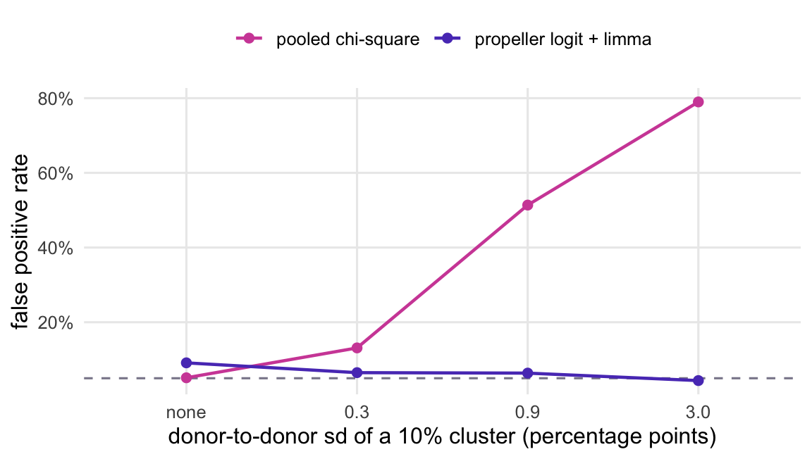
The pooled tests would be fine if donors did not differ. Figure 3 repeats the null run with 3 donors per condition and less donor variation, 100 experiments per level. When every donor’s cells are sampled from the same proportions, the pooled chi-square test gives p < 0.05 in 5.1% of comparisons. At a donor-to-donor standard deviation of 0.3 percentage points for a cluster with a 10% share, it is 13%; at 0.9 points, 51%; at the 3.0 points used above, 79%. The propeller transformation stays between 4.4% and 9.1% throughout.
The reason is the scale of the noise each test expects. For a 10% cluster and about 18,000 cells per condition, the binomial sampling noise the pooled test allows for has a standard deviation of about 0.2 percentage points. Donor differences of that order already inflate its false positive rate, and more cells per donor make the expected noise smaller while the donor differences stay the same.
Figure 3: False positive rate averaged over clusters, three versus three donors, as donors differ more in composition. The horizontal axis gives the donor-to-donor standard deviation of a cluster that makes up 10% of cells, in percentage points.
             method design       rate
1             chisq 3 vs 3 0.92142857
2          edgeR_QL 3 vs 3 0.23571429
3      edgeR_QL_TMM 3 vs 3 0.08809524
4  edgeR_QL_without 3 vs 3 0.06904762
5   propeller_logit 3 vs 3 0.27142857
6             chisq 6 vs 6 0.94047619
7          edgeR_QL 6 vs 6 0.41904762
8      edgeR_QL_TMM 6 vs 6 0.08095238
9  edgeR_QL_without 6 vs 6 0.03571429
10  propeller_logit 6 vs 6 0.44285714
Now one real change: C2 triples in treated donors, and the cells of every other cluster are left alone. Because the shares of a sample add up to one, the expected share of each of the other 7 clusters in treated donors falls to 71% of its baseline, while C2 goes from 20% to 43%. This is the compositional effect: a test of proportions sees every cluster change. Whether that is wrong depends on the question. If you want to know whether the share of C3 changed, it did. If you want to know whether C3 cells became more or less numerous in the tissue, the proportions cannot tell you, because the number of cells in a sample is set by how many were loaded, not by the tissue. The post on correlations of proportions covers the same constraint from another angle.
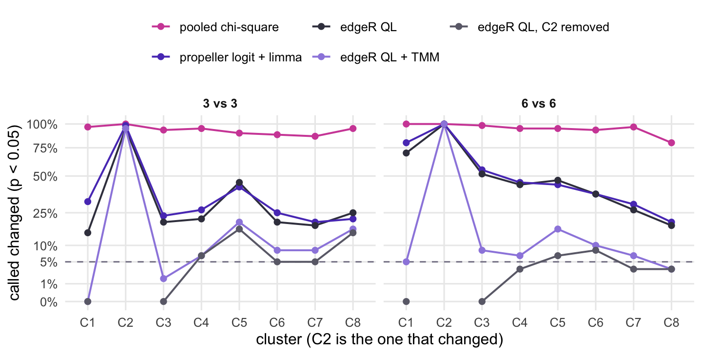
Figure 4 has the result over 60 experiments per design. Every method calls C2 in at least 95% of experiments. The pooled chi-square test calls the untouched clusters in 92% of comparisons with 3 donors per condition, up from 81% with no change at all. The donor-level tests call them in 27% (propeller) and 24% (edgeR), and in 44% and 42% with 6 donors per condition: with more donors, the real drop in share becomes easier to detect.
The OSCA chapter offers two fixes, each resting on an assumption. TMM normalisation (normLibSizes(), as in the post on library size and composition) assumes that most clusters do not change and rescales each donor so that the typical cluster is flat. The untouched clusters are then called in 8.8% and 8.1% of comparisons (3 and 6 donors per condition): far less often than without it, but above the 6.2% and 5.9% the same edgeR test gives when nothing changes. The rescaling is itself estimated from a few clusters, and it does not remove the effect completely. Removing the cluster that obviously moved and testing the rest, with library sizes recomputed from the remaining clusters, gives 6.9% and 3.6%. Both rest on an assumption the counts cannot check: TMM that most clusters are stable, removal that you know which cluster moved. With one change among 8 clusters it holds here by construction; with four cell types of which two change, it would not.
Compositional models build the constraint into the model instead: scCODA (Buttner et al. 2021) reports changes relative to a reference cell type that is assumed not to change (its reference_cell_type argument), and the Bioconductor package sccomp is another option in this family. Neither is run here.
exp_lab <-c(chisq ="pooled chi-square", propeller_logit ="propeller logit + limma",edgeR_QL ="edgeR QL", edgeR_QL_TMM ="edgeR QL + TMM",edgeR_QL_without ="edgeR QL, C2 removed")exp_col <-setNames(c(magenta, violet, "#3d3d4d", "#9d8ae0", "#6b6b78"), exp_lab)flag$method_lab <-factor(exp_lab[flag$method], levels = exp_lab)flag$cluster <-factor(flag$cluster, levels =names(base_prop))# the "C2 removed" line has no C2 value: draw it in two pieces instead of across C2flag$piece <-paste(flag$method, flag$method =="edgeR_QL_without"&as.integer(flag$cluster) >match(target, names(base_prop)))ggplot(flag, aes(cluster, rate, colour = method_lab, group = piece)) +geom_hline(yintercept = alpha, linetype ="dashed", colour = grey) +geom_line(linewidth =0.7) +geom_point(size =1.8) +scale_y_sqrt(breaks =c(0, 0.01, 0.05, 0.1, 0.25, 0.5, 0.75, 1),labels =function(v) paste0(100* v, "%")) +scale_colour_manual(values = exp_col) +facet_wrap(~ design) +labs(x ="cluster (C2 is the one that changed)", y =paste0("called changed (p < ", alpha, ")"),colour =NULL) +theme(legend.position ="top") +guides(colour =guide_legend(nrow =2))
Figure 4: One cluster (C2) is expanded in treated donors and nothing else changes. The lines give how often each cluster is called changed at the significance threshold; for every cluster except C2, a call is a compositional side effect. Square-root vertical axis.
The script below runs the pooled chi-square test the way a scanpy user often does, from a crosstab of the cell metadata in adata.obs, against a donor-level test in statsmodels: a binomial GLM per cluster whose scale is estimated from the Pearson chi-square (a quasi-binomial model), with t-tests on the residual degrees of freedom. It simulates 200 tables per design the same way, with numpy’s random generator, so the draws and the exact numbers differ from the R run. The numbers were computed with statsmodels 0.15.0 and scipy 1.17.1 and are shown for comparison. The pooled chi-square test gave p < 0.05 in 82% and 83% of null comparisons (3 vs 3 and 6 vs 6 donors); the quasi-binomial GLM gave 5.9% and 6.3%.
One trap on the way. In statsmodels 0.15.0, a binomial GLM accepts a two-column response (successes, failures), but with that form and scale="X2", the scale it estimated on the example table was 0.017, against 78.0 for the Pearson chi-square divided by the residual degrees of freedom computed by hand. The fit’s own pearson_chi2 / df_resid gives the right value (78.0), so the problem is only in the scale used for the standard errors, and a scale that small makes the test far too liberal. A quasi-binomial scale below 1 on counts from several donors is a warning sign in itself. Passing the proportions as the response with the cell totals as var_weights gives 78.0, the quasi-binomial value. The crosstab route and a route that sums counts per condition give the same chi-square p-values (largest difference 0.0).
"""Cell type proportions in Python: pooled chi-square vs a donor-level quasi-binomial GLM.Simulates donor x cluster tables the same way as the R code in the post (Dirichlet donorproportions around a common baseline, multinomial cell counts), with no true condition effect,and counts how often each test gives p < 0.05. Writes proportion_check-results.csv."""import numpy as npimport pandas as pdimport scipyimport statsmodelsimport statsmodels.api as smfrom scipy.stats import chi2_contingencyrng = np.random.default_rng(2026)base_prop = np.array([0.30, 0.20, 0.15, 0.10, 0.08, 0.07, 0.06, 0.04])clusters = [f"C{i +1}"for i inrange(len(base_prop))]conc =100# Dirichlet concentration: donor-to-donor variation in compositionalpha =0.05n_tables =200# replicate tables per designdef simulate_table(n_per_group):"""Donor x cluster cell counts with no true condition effect.""" n =2* n_per_group totals = rng.integers(2000, 10001, size=n) props = rng.dirichlet(base_prop * conc, size=n) counts = np.vstack([rng.multinomial(t, p) for t, p inzip(totals, props)]) condition = np.repeat(["ctrl", "trt"], n_per_group)return counts, conditiondef to_obs(counts, condition):"""Expand a donor x cluster table into a cell-level table like adata.obs.""" rows = []for d inrange(counts.shape[0]):for k, c inenumerate(clusters): rows.append(pd.DataFrame({"donor": f"d{d +1:02d}", "condition": condition[d],"cluster": [c] *int(counts[d, k])}))return pd.concat(rows, ignore_index=True)def pooled_chisq(obs):"""The common route: crosstab of cells, then one 2 x 2 test per cluster.""" tab = pd.crosstab(obs["cluster"], obs["condition"]) tot = tab.sum(axis=0)return np.array([chi2_contingency(np.vstack([tab.loc[c], tot - tab.loc[c]]))[1]for c in clusters])def quasi_binomial(counts, condition):"""Donor-level test: binomial GLM per cluster with a Pearson chi-square scale.""" x = sm.add_constant((condition =="trt").astype(float)) totals = counts.sum(axis=1) p = []for k inrange(counts.shape[1]):# response as proportions, cell totals as var_weights: a two-column response# gives a much smaller Pearson scale in statsmodels 0.15 (see scales() below) fit = sm.GLM(counts[:, k] / totals, x, family=sm.families.Binomial(), var_weights=totals).fit(scale="X2", use_t=True) p.append(fit.pvalues[1])return np.array(p)def scales(counts, condition, k=0):"""Estimated scale for one cluster: two-column response vs proportions + var_weights, and the quasi-binomial scale computed by hand (Pearson chi-square / residual df).""" x = sm.add_constant((condition =="trt").astype(float)) totals = counts.sum(axis=1) two_col = sm.GLM(np.column_stack([counts[:, k], totals - counts[:, k]]), x, family=sm.families.Binomial()).fit(scale="X2") weighted = sm.GLM(counts[:, k] / totals, x, family=sm.families.Binomial(), var_weights=totals).fit(scale="X2") mu = weighted.fittedvalues pearson = np.sum(totals * (counts[:, k] / totals - mu) **2/ (mu * (1- mu)))return (two_col.scale, two_col.pearson_chi2 / two_col.df_resid, weighted.scale, pearson / weighted.df_resid)# one table through the cell-level (obs) route, checked against the fast count routecounts, condition = simulate_table(3)obs = to_obs(counts, condition)p_obs = pooled_chisq(obs)fast = pd.DataFrame(counts, columns=clusters)fast["condition"] = conditionsummed = fast.groupby("condition")[clusters].sum().Tp_fast = np.array([chi2_contingency(np.vstack([summed.loc[c], summed.sum() - summed.loc[c]]))[1]for c in clusters])route_diff =float(np.max(np.abs(p_obs - p_fast)))scale_two_col, pearson_two_col, scale_weighted, scale_by_hand = scales(counts, condition)results = {"n_cells_example": len(obs), "route_max_abs_diff": route_diff,"scale_two_col": scale_two_col, "pearson_df_two_col": pearson_two_col,"scale_weighted": scale_weighted,"scale_by_hand": scale_by_hand,"n_tables": n_tables, "n_clusters": len(clusters)}for npg in (3, 6): chi, qb = [], []for _ inrange(n_tables): counts, condition = simulate_table(npg) s = pd.DataFrame(counts, columns=clusters).groupby(condition).sum().T chi.append([chi2_contingency(np.vstack([s.loc[c], s.sum() - s.loc[c]]))[1]for c in clusters]) qb.append(quasi_binomial(counts, condition)) results[f"fpr_chisq_{npg}v{npg}"] =float(np.mean(np.array(chi) < alpha)) results[f"fpr_quasibinom_{npg}v{npg}"] =float(np.mean(np.array(qb) < alpha))results["numpy_version"] = np.__version__results["pandas_version"] = pd.__version__results["scipy_version"] = scipy.__version__results["statsmodels_version"] = statsmodels.__version__pd.DataFrame({"name": list(results), "value": list(results.values())}).to_csv("proportion_check-results.csv", index=False)print(pd.Series(results))
What to do in practice
Build the table of cells per donor and cluster, and test at the donor level. With a Seurat object (or as.data.frame(colData(sce)) for a SingleCellExperiment) whose metadata has donor, condition and cluster columns, and the two functions defined above:
meta <- so[[]] # cell metadatacounts <-unclass(table(meta$donor, meta$cluster)) # donors x clustersgroup <-factor(meta$condition[match(rownames(counts), meta$donor)])p <-propeller_like(counts, group) # or edger_da(counts, group)p.adjust(p, "BH") # across clusters
The packaged version is speckle::propeller(clusters = , sample = , group = ), one value per cell; its defaults in the speckle source are transform = "logit", robust = TRUE and trend = FALSE. For a design with covariates such as batch, speckle also exports getTransformedProps(), which builds the transformed table, and propeller.ttest(), which fits it with a design matrix and a contrast.
Count donors, not cells, when you plan the experiment. With two donors per condition, each cluster’s test has two residual degrees of freedom; in the simulation above, with three, the donor-level tests were least well calibrated for the rare clusters.
Before reading the list of changed clusters, decide whether the question is about shares or about numbers of cells. If one cell type expands, the shares of the others fall. Report them as shares, or use a fix whose assumption you can defend (most clusters stable, or a known reference), or a compositional model. An answer about numbers of cells in the tissue needs information the sequencing does not have, such as cell counts per amount of tissue from another assay.