Is it fine to treat cells as replicates in single-cell differential expression? A simulation of Wilcoxon cell-level tests against pseudobulk edgeR and DESeq2.
You have single-cell RNA-seq data from treated and control samples and you want the genes that respond to treatment. The quickest route is to put all treated cells in one group and all control cells in the other, then test gene by gene. In Seurat that is FindMarkers(), whose default is a Wilcoxon rank-sum test on log-normalised expression. So the question people type into a search box is: can I treat cells as replicates?
Not when the conditions come from different donors (or mice, or cultures). In the simulation below, with 3 donors per condition and 300 cells per donor, the cell-level Wilcoxon test gave p < 0.05 for 54% of the genes that have no true effect. Summing the counts per donor first (a pseudobulk) and testing with edgeR gave 4.4%, close to the 5% a p < 0.05 threshold promises.
The setup
simulate_sc <-function(n_genes =2000, n_de =200, donors_per_group =3,cells_per_donor =300, donor_sd =0.3, lfc =1, phi =0.3) { n_donor <-2* donors_per_group donor <-factor(rep(sprintf("d%d", seq_len(n_donor)), each = cells_per_donor)) donor_group <-factor(rep(c("ctrl", "trt"), each = donors_per_group)) group <- donor_group[as.integer(donor)] mu <-exp(rnorm(n_genes, log(0.5), 1)) # baseline mean UMI per cell is_de <-seq_len(n_genes) <= n_de # the first n_de genes truly change beta <-ifelse(is_de, sample(c(-1, 1), n_genes, replace =TRUE) * lfc *log(2), 0) b <-matrix(rnorm(n_genes * n_donor, 0, donor_sd), n_genes, n_donor) # donor effects size <-exp(rnorm(length(donor), 0, 0.3)) # cell-to-cell capture efficiency trt <-as.numeric(group =="trt") m <- mu *exp(b[, as.integer(donor)] +outer(beta, trt)) m <-sweep(m, 2, size, "*") counts <-matrix(rnbinom(length(m), mu = m, size =1/ phi), n_genes)dimnames(counts) <-list(sprintf("g%04d", seq_len(n_genes)),sprintf("c%05d", seq_along(donor)))list(counts = counts, donor = donor, group = group, is_de = is_de)}set.seed(1)sim <-simulate_sc()n_genes <-nrow(sim$counts); n_de <-sum(sim$is_de); n_null <- n_genes - n_den_cells <-ncol(sim$counts); cells_per_donor <- n_cells /nlevels(sim$donor)n_per_group <-formals(simulate_sc)$donors_per_groupdonor_sd_main <-formals(simulate_sc)$donor_sddonor_shift <-exp(donor_sd_main) -1# one sd up, as a ratiodonor_shift_down <-1-exp(-donor_sd_main) # one sd downfold <-2^formals(simulate_sc)$lfcshare_low <-mean(rowMeans(sim$counts) <1)
The simulated experiment is one cell type from 6 donors, 3 control and 3 treated, with 300 cells each (1,800 cells in total) and 2,000 genes. Counts follow a negative binomial distribution, the usual model for UMI counts. Each gene’s expression is built from a baseline level (72% of genes average less than one UMI per cell, a few average many), a donor effect, and cell-to-cell noise that includes differences in how many molecules each cell captured.
The donor effect is the assumption that matters. Each donor’s level of each gene is shifted up or down at random, with a standard deviation of 0.3 on the natural log scale: one standard deviation puts a donor about 35% above or 26% below the average for a given gene. Real donors differ like this for reasons unrelated to the treatment, such as genotype or the time from sampling to dissociation. How large the effect is depends on the tissue and the organism (inbred mice usually vary less than human donors), so the sweep further down also runs the case with no donor variation at all.
The first 200 genes get a true treatment effect, a 2-fold change up or down. The other 1,800 genes have no treatment effect, so any of them that a test calls significant is a false positive.
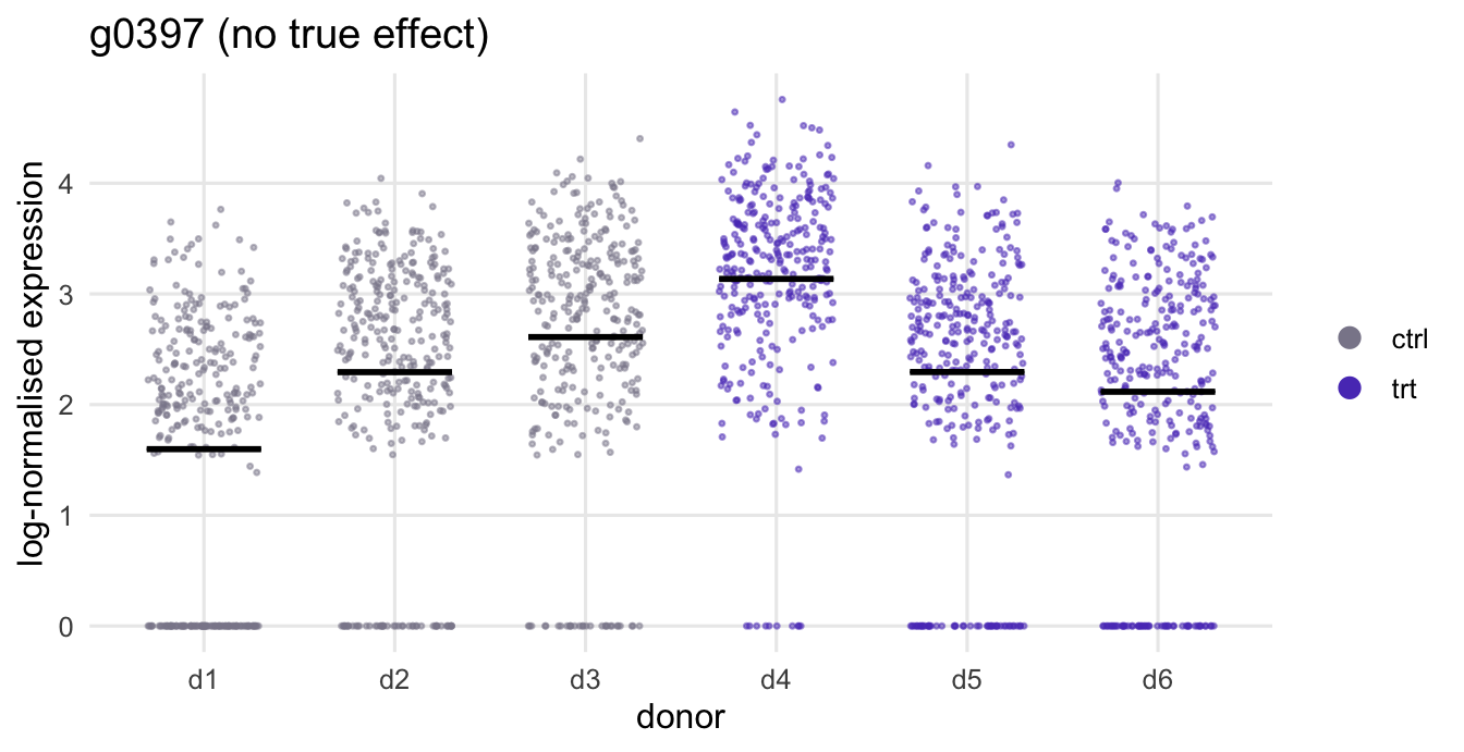
Figure 1 shows what the donor effect looks like for one gene with no true effect. It is not the worst case: among the well-expressed null genes it is the one at the 90th percentile of the gap between treated and control donor means.
so <-CreateSeuratObject(as(sim$counts, "CsparseMatrix"),meta.data =data.frame(donor = sim$donor, group = sim$group,row.names =colnames(sim$counts)))so <-NormalizeData(so, verbose =FALSE) # LogNormalize, scale factor 1e4lognorm <-as.matrix(GetAssayData(so, layer ="data"))# a well-expressed null gene whose donor means happen to separate by conditionnull_ids <-which(!sim$is_de &rowMeans(sim$counts) >2)donor_means <-sapply(split(seq_len(n_cells), sim$donor),function(j) rowMeans(lognorm[null_ids, j, drop =FALSE]))gap <-rowMeans(donor_means[, 4:6]) -rowMeans(donor_means[, 1:3])# not the most extreme gene: the one at the 90th percentile of the treated-minus-control gappick_q <-0.9gene_show <-names(gap)[which.min(abs(gap -quantile(gap, pick_q)))]
Figure 1: One gene with no true condition effect. Each column of points is one donor’s cells; the black bar is that donor’s mean. The cells of a donor share that donor’s level, so the treated donors can sit above the controls by chance.
formals() on the installed Seurat returns “wilcox” as the default test.use, the Wilcoxon rank-sum test. Two other defaults drop genes before any test is run, logfc.threshold (0.1 in this version) and min.pct; both are set to zero above so that every gene gets a p-value and the false positive rate is measured on all of them. densify = TRUE only changes the speed. If the presto package is installed, Seurat runs the same test through presto’s faster implementation, which computes the same statistic with the same tie and continuity corrections.
For the gene in Figure 1, the cell-level test gives p = 5.5e-11. It compares 900 treated cells with 900 control cells, and with that many observations even a small shift between the two sets counts as overwhelming evidence. (The +1 inside the log-normalisation is a pseudocount, which also affects log fold changes; see the pseudocount post.)
The pseudobulk is a plain sum: AggregateExpression() adds up the raw counts of each donor’s cells (its result matches rowsum() on the count matrix; largest difference 0). That leaves 6 samples, one per donor, which is what a bulk RNA-seq tool expects. edgeR runs with its quasi-likelihood recipe (filterByExpr, normLibSizes, glmQLFit with robust = TRUE, glmQLFTest; Chen et al. 2016) and DESeq2 with its standard DESeq() and results() (Love et al. 2014). legacy = FALSE selects the quasi-likelihood method added in edgeR 4.0; it is set explicitly so that older and newer edgeR versions run the same method. For the gene in Figure 1, pseudobulk edgeR gives p = 0.15.
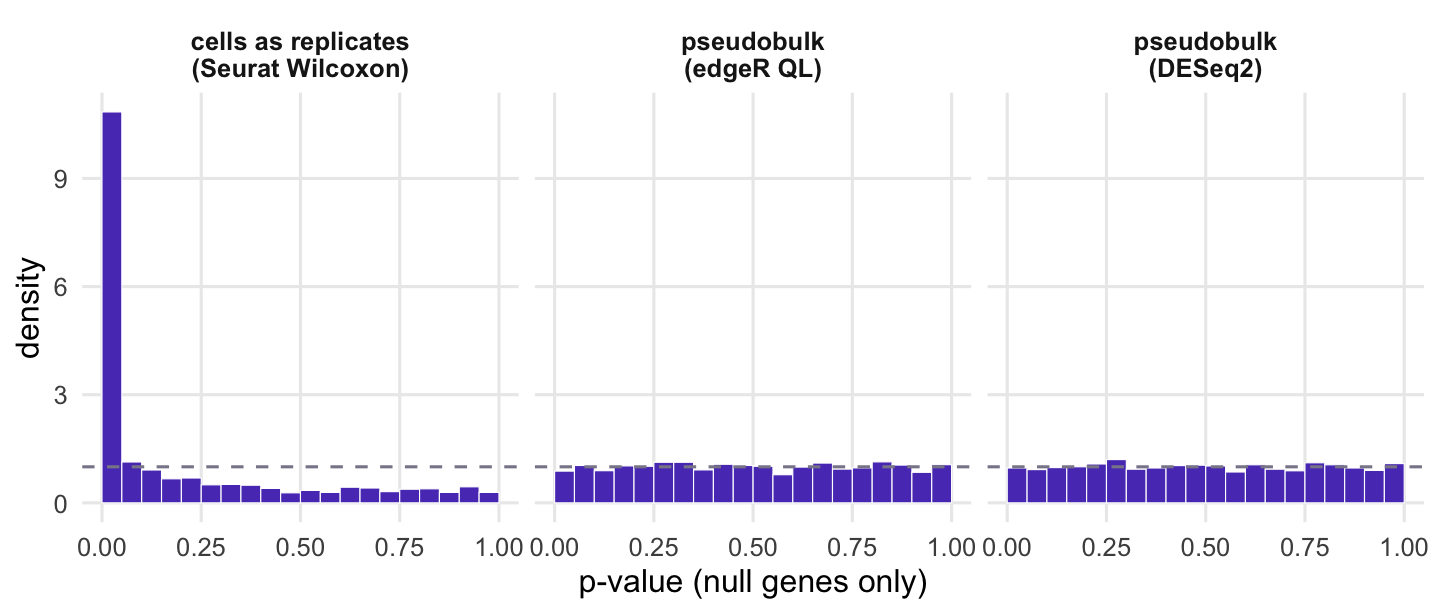
Across all 1,800 null genes, the cell-level test gave p < 0.05 for 976 of them, a false positive rate of 54%, about 11 times the nominal rate. The pseudobulk tests gave 4.4% (edgeR, on the genes that pass filterByExpr) and 4.8% (DESeq2). Figure 2 shows the same thing as p-value histograms: for genes with no effect, a calibrated test gives a flat histogram, and the cell-level test does not.
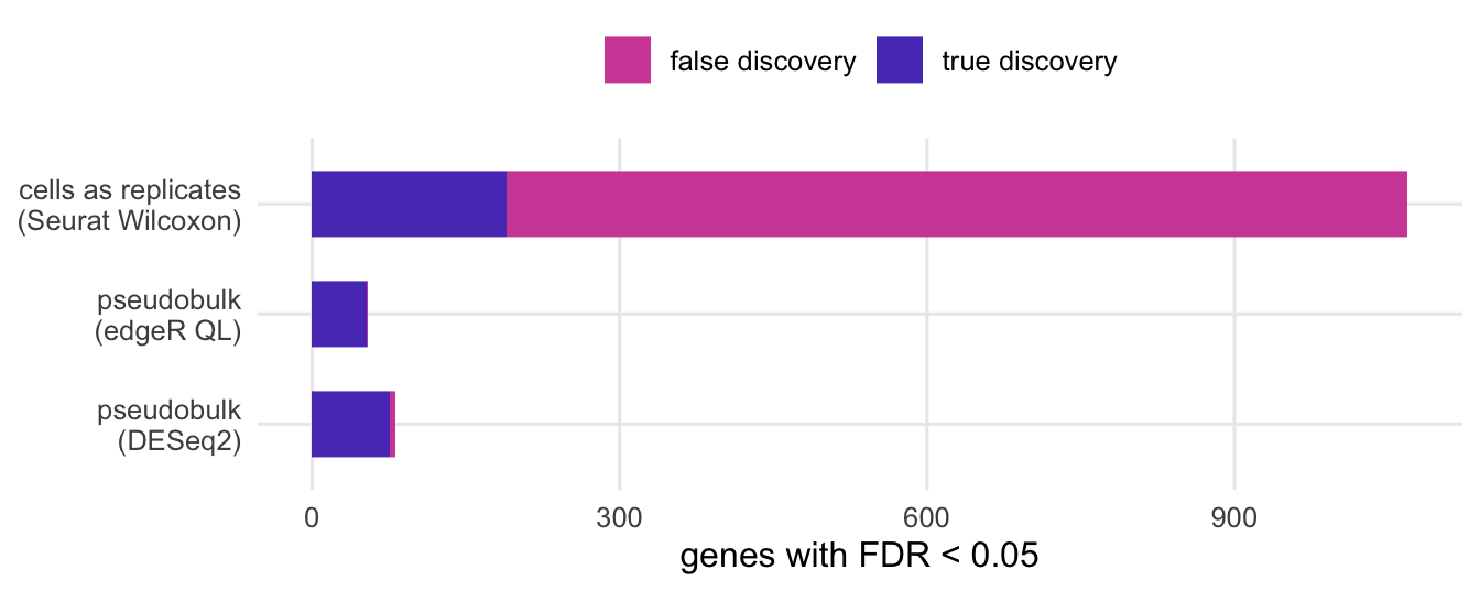
What people act on is the list of significant genes. At a Benjamini-Hochberg FDR of 5%, the cell-level test reported 1,069 genes, of which 879 are null: an observed false discovery rate of 82% where 5% was promised. Seurat’s own p_val_adj column uses a Bonferroni correction over all genes, which is much stricter, and it still let through 367 null genes. The false discoveries from pseudobulk numbered 1 with edgeR and 5 with DESeq2 (Figure 3).
The price is sensitivity. The cell-level test found 190 of the 200 truly changed genes; pseudobulk edgeR found 53 and DESeq2 76. With 3 donors per group, there is little information about how much donors vary, and a 2-fold change is often not distinguishable from donor noise. That is an accurate statement of what 3 donors can tell you. The cell-level test’s extra hits cannot be used, because they arrive mixed with 879 false ones and nothing in the output says which are which.
Figure 2: P-values of the genes with no true effect. Under a well-calibrated test they spread evenly between 0 and 1 (dashed line). The cell-level Wilcoxon test piles them up near zero; both pseudobulk tests stay close to flat.
dd <-data.frame(method =factor(rep(lab, 2), levels =rev(lab)),kind =factor(rep(c("true discovery", "false discovery"), each =3),levels =c("false discovery", "true discovery")),n =c(tab[, "td"], tab[, "fd"]))ggplot(dd, aes(n, method, fill = kind)) +geom_col(width =0.6) +scale_fill_manual(values =c("true discovery"= violet, "false discovery"= magenta)) +labs(x =paste("genes with FDR <", alpha), y =NULL, fill =NULL) +theme(legend.position ="top")
Figure 3: Genes called significant at the Benjamini-Hochberg FDR threshold used in the text, split into truly changed genes and genes with no effect. The cell-level test finds almost every true gene and many more false ones.
Why more cells make it worse
# Wilcoxon rank-sum test with tie correction and continuity correction (normal# approximation), the same test FindMarkers runs, vectorised for the sweep below.wilcox_rows <-function(x, in2) { n2 <-sum(in2); n1 <-length(in2) - n2; n <- n1 + n2vapply(seq_len(nrow(x)), function(i) { r <-rank(x[i, ]) ties <-tabulate(match(r, unique(r))) u <-sum(r[in2]) - n2 * (n2 +1) /2 s <-sqrt(n1 * n2 /12* ((n +1) -sum(ties^3- ties) / (n * (n -1)))) z <- (abs(u - n1 * n2 /2) -0.5) / smin(2*pnorm(z, lower.tail =FALSE), 1) }, numeric(1))}p_check <-wilcox_rows(lognorm, sim$group =="trt")wilcox_diff <-max(abs(p_check - p_cell))wilcox_diff
The cell-level test asks whether treated cells rank higher than control cells, and treats every cell as an independent observation. It answers that question correctly: these particular 900 treated cells do differ from these 900 control cells, because their donors differ. But the experiment asks whether the treatment changes expression in the population the donors came from, and for that question the replicates are the donors. There are 3 per group, however many cells each one contributes.
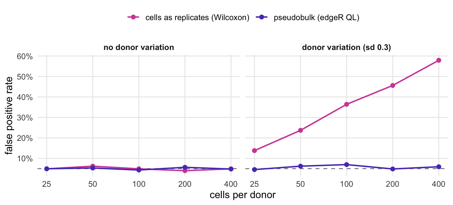
This predicts that more cells per donor should make the cell-level test worse, not better, and that without donor variation it should be fine. To check, the helper wilcox_rows() above reproduces the FindMarkers() p-values (largest absolute difference 3e-16) and is fast enough to rerun on 10 simulated data sets (one for each combination of cell count and donor variation in Figure 4), each with 3 donors per group and 1,000 null genes.
Figure 4 has the result. With no donor variation, the cell-level test stays calibrated: its false positive rate is close to the nominal rate, at most 6.2% at any cell count. With donor variation it climbs from 14% at 25 cells per donor to 58% at 400. Pseudobulk edgeR stays between 4.3% and 7.0% throughout, because summing more cells makes each donor’s total more precise without pretending there are more donors.
Figure 4: False positive rate on genes with no effect as the number of cells per donor grows. Left: donors identical apart from cell-level noise. Right: donors differ. The dashed line is the nominal rate.
The script below runs the same comparison in scanpy and PyDESeq2 on an AnnData object simulated the same way, with numpy’s random generator (so the draws, and the exact numbers, differ from the R run). The numbers were computed with scanpy 1.11.5 and PyDESeq2 0.5.4 and are shown for comparison. sc.tl.rank_genes_groups(..., method="wilcoxon") gave p < 0.05 for 46% of null genes; pseudobulk with PyDESeq2 gave 6.9%, a little above the nominal 5%. At an FDR of 5%, scanpy reported 728 false and 187 true discoveries, PyDESeq2 7 false and 73 true. The script also reruns the pseudobulk step on four more simulated data sets: across all 5, PyDESeq2’s false positive rate ranged from 5.9% to 6.9%. That is consistently a little above the nominal rate in this setup, and above the R DESeq2 run, but still far below the cell-level test. The cause was not traced here, so treat it as a difference between the two implementations at 3 samples per group rather than a property of pseudobulk. One difference from Seurat: scanpy’s Wilcoxon skips the correction for tied values by default (tie_correct=False), and single-cell data are full of tied zeros. Without the correction the test is more conservative; with it switched on, the false positive rate on the same data was 55%. Either way the problem is the same.
# Cells as replicates vs pseudobulk, in scanpy + PyDESeq2.# Same design as the R code in the post: 3 vs 3 donors, donor-level variation, 10% true DE genes.# Writes pseudobulk_check-results.csv (columns name,value).from importlib.metadata import versionimport anndata as adimport numpy as npimport pandas as pdimport scanpy as scfrom pydeseq2.dds import DeseqDataSetfrom pydeseq2.ds import DeseqStatsn_genes, n_de, per_group, cells_per_donor =2000, 200, 3, 300donor_sd, phi, alpha =0.3, 0.3, 0.05n_donor =2* per_groupis_de = np.arange(n_genes) < n_dedef simulate(rng): donor = np.repeat([f"d{i +1}"for i inrange(n_donor)], cells_per_donor) group = np.repeat(np.repeat(["ctrl", "trt"], per_group), cells_per_donor) mu = np.exp(rng.normal(np.log(0.5), 1.0, n_genes)) # baseline mean per cell beta = np.where(is_de, rng.choice([-1.0, 1.0], n_genes) * np.log(2), 0.0) b = rng.normal(0.0, donor_sd, (n_donor, n_genes)) # donor effects size = np.exp(rng.normal(0.0, 0.3, donor.size)) # cell size factors d_idx = np.repeat(np.arange(n_donor), cells_per_donor) trt = (group =="trt").astype(float) m = size[:, None] * mu[None, :] * np.exp(b[d_idx] + trt[:, None] * beta[None, :]) counts = rng.poisson(m * rng.gamma(1.0/ phi, phi, m.shape)) # negative binomial adata = ad.AnnData( X=counts.astype(np.float32), obs=pd.DataFrame({"donor": donor, "group": group}, index=[f"c{i +1:05d}"for i inrange(donor.size)]), var=pd.DataFrame(index=[f"g{i +1:04d}"for i inrange(n_genes)]), ) adata.layers["counts"] = adata.X.copy() # keep raw countsreturn adatadef pseudobulk_deseq(adata):# sum RAW counts per donor, then PyDESeq2 pb = sc.get.aggregate(adata, by="donor", func="sum", layer="counts") counts = pd.DataFrame(np.rint(pb.layers["sum"]).astype(int), index=pb.obs_names, columns=adata.var_names) donor_group = adata.obs.groupby("donor", observed=True)["group"].first() meta = pd.DataFrame({"group": donor_group.loc[counts.index].to_numpy()}, index=counts.index) dds = DeseqDataSet(counts=counts, metadata=meta, design="~group", quiet=True, n_cpus=1) dds.deseq2() st = DeseqStats(dds, contrast=["group", "trt", "ctrl"], quiet=True, n_cpus=1) st.summary() res = st.results_df.loc[adata.var_names]return res["pvalue"].to_numpy(), res["padj"].to_numpy()def fpr(p): ok =~is_de &~np.isnan(p)returnfloat(np.mean(p[ok] < alpha))def count(q, which):returnint(np.sum((q < alpha) & which &~np.isnan(q)))adata = simulate(np.random.default_rng(2026))genes = adata.var_names# Cells as replicates: Wilcoxon on log-normalised expressioncell = adata.copy()sc.pp.normalize_total(cell, target_sum=1e4)sc.pp.log1p(cell)sc.tl.rank_genes_groups(cell, "group", groups=["trt"], reference="ctrl", method="wilcoxon")w = sc.get.rank_genes_groups_df(cell, group="trt").set_index("names").loc[genes]p_w, q_w = w["pvals"].to_numpy(), w["pvals_adj"].to_numpy()# scanpy skips the tie correction by default (tie_correct=False); Seurat applies itsc.tl.rank_genes_groups(cell, "group", groups=["trt"], reference="ctrl", method="wilcoxon", tie_correct=True, key_added="wilcoxon_ties")wt = sc.get.rank_genes_groups_df(cell, group="trt", key="wilcoxon_ties").set_index("names")p_wt = wt.loc[genes, "pvals"].to_numpy()# Pseudobulk + PyDESeq2p_d, q_d = pseudobulk_deseq(adata)# PyDESeq2 false positive rate on four more simulated data setsextra = [fpr(pseudobulk_deseq(simulate(np.random.default_rng(s)))[0]) for s in (1, 2, 3, 4)]all_d = [fpr(p_d)] + extrarows = {"fpr_wilcoxon": fpr(p_w),"fpr_wilcoxon_tiecorr": fpr(p_wt),"fpr_pydeseq2": fpr(p_d),"false_disc_wilcoxon": count(q_w, ~is_de),"false_disc_pydeseq2": count(q_d, ~is_de),"true_disc_wilcoxon": count(q_w, is_de),"true_disc_pydeseq2": count(q_d, is_de),"n_de": n_de,"n_null": int(np.sum(~is_de)),"pydeseq2_n_datasets": len(all_d),"fpr_pydeseq2_min": min(all_d),"fpr_pydeseq2_max": max(all_d),"scanpy_version": version("scanpy"),"pydeseq2_version": version("pydeseq2"),}pd.DataFrame({"name": list(rows), "value": list(rows.values())}).to_csv("pseudobulk_check-results.csv", index=False)print(pd.Series(rows))
What to do in practice
Decide what the replicate is before you analyse anything. It is the unit that was independently assigned to a condition or sampled from the population, such as a donor or an animal. Cells inside it are measurements of that unit, the way technical replicates are in a bulk experiment.
For differential expression between conditions, sum the raw counts per sample within each cell type, then run a bulk method the way its authors recommend. In Seurat, the loop looks like this (celltype, donor and condition are metadata columns you already have):
for (ct inunique(so$celltype)) { sub <-subset(so, celltype == ct) pb <-as.matrix(AggregateExpression(sub, group.by ="donor",return.seurat =FALSE)$RNA)# AggregateExpression() may rewrite group names (for example, adding a "g" before a# leading digit), so check that every column found its donor condition <- sub$condition[match(colnames(pb), sub$donor)]stopifnot(!anyNA(condition))# ... then the edgeR block above, with condition in place of pb_group}
In scanpy, sc.get.aggregate(adata, by=["celltype", "donor"], func="sum", layer="counts") does the summing (the sums land in .layers["sum"]); the counts layer must hold raw counts, not the log-normalised values that X usually holds after preprocessing. The script above uses the same call with by="donor". If each donor contributes both conditions (before and after treatment, say), put the donor in the design, ~ donor + condition, so the comparison is made within donors. The muscat package wraps pseudobulk aggregation per cluster and also offers cell-level mixed models, which keep the cells but model the donor as a random effect (Crowell et al. 2020).
Keep cell-level tests for questions that really are about the cells in hand, such as which genes separate one cluster from another in the same samples. Seurat’s own differential expression vignette makes the same point, noting that these tests treat each cell as an independent replicate, and shows a pseudobulk alternative. A large benchmark reached the same conclusion: methods that ignore variation between biological replicates find hundreds of genes in data with no biological difference (Squair et al. 2021).
If pseudobulk gives you too few genes, the fix is more donors. Adding cells per donor does not add replicates.