Proportions of independent taxa or cell types still correlate. A simulation of spurious correlation in relative abundance data and what CLR and rho can fix.
You have a table of relative abundances, bacterial taxa from 16S sequencing or cell types from a single-cell atlas, and you want to know which ones go together. The obvious move is cor() on the proportions, followed by a network of the strongest pairs. The question is whether a correlation between two proportions says anything about the two organisms or cell types themselves.
Often it does not. Proportions are shares of a total, and shares are tied to each other whatever the biology does. In the simulation below, 30 taxa have absolute abundances that are completely independent of each other. Yet 11.1% of taxon pairs show a correlation of proportions with , where a correct test gives 5% (the absolute abundances give 5.2%). The most abundant taxon is negatively correlated with 95% of the others, with a median correlation of -0.22. Here, taking logs of the proportions makes it worse, not better.
Why proportions cannot be independent
In every sample the proportions add up to 1. A quantity that never varies has zero covariance with anything, so for any part the covariance of with the total is zero, and splitting the total into its parts gives
Each part’s covariances with the others must add up to minus its own variance. That is an identity, not an estimate: if one part goes up, the others must, taken together, go down by the same amount. So the correlations of proportions cannot all be zero even when the underlying abundances have nothing to do with each other. Data with this property are called compositional, and dividing by the total is called closure.
Sequencing makes almost every abundance table compositional. The number of reads per sample is set by the sequencer, not by how many cells were in the tube, so only the relative amounts carry information. Gloor et al. (2017) make this case for microbiome data. The same applies to cell-type proportions from single-cell data, where the total is the number of cells captured.
The setup
clr <-function(x) log(x) -rowMeans(log(x)) # rows = samples, columns = partsrho <-function(z) { # z: CLR-transformed matrix v <-apply(z, 2, var)2*cov(z) /outer(v, v, "+") # = 1 - var(z_i - z_j) / (var z_i + var z_j)}lr_var <-function(x) { # variance of log(x_i / x_j), all pairs l <-log(x); v <-apply(l, 2, var)outer(v, v, "+") -2*cov(l)}pairs_of <-function(m) m[upper.tri(m)] # one value per paircor_p <-function(r, n) { # two-sided p-value of the usual t test2*pt(-abs(r *sqrt((n -2) / (1- r^2))), n -2)}
Each simulated data set has 50 samples and 30 taxa. The absolute abundance of every taxon in every sample is drawn independently from a log-normal distribution with a standard deviation of 1 on the natural log scale, so the true correlation between any two taxa is zero. The taxa differ in typical size along a steep curve (a Zipf curve with exponent 1.5, so the typical size of the -th largest taxon falls as to the power -1.5), and on average the largest one holds 37% of each sample. Each sample is then sequenced: a number of reads between 5,000 and 50,000 is drawn from the true proportions. Only 0.2% of the resulting counts are zero.
n_samples <-50; n_taxa <-30; sd_log <-1; zipf <-1.5depth_range <-c(5000, 50000); pc_main <-0.5zipf_shares <-function(D, a) { s <-seq_len(D)^-a; s /sum(s) }simulate_community <-function(shares, n = n_samples, depth = depth_range) { D <-length(shares)# absolute abundances: independent log-normal, one column per taxon A <-exp(matrix(rnorm(n * D, mean =rep(log(shares), each = n), sd = sd_log), n, D)) P <- A /rowSums(A) # true proportions reads <-round(exp(runif(n, log(depth[1]), log(depth[2])))) Y <-t(vapply(seq_len(n), function(i) rmultinom(1, reads[i], P[i, ])[, 1], numeric(D)))list(A = A, P = P, Y = Y, reads = reads)}
Three assumptions matter. Independence of the absolute abundances is the truth being tested, so any correlation that comes out is spurious. Every taxon has the same variance on the log scale; this makes the arithmetic further down exact, and real taxa vary in variability. And one taxon dominates, which the next sections vary on purpose.
The analysis is repeated on 200 data sets, giving 87,000 pairwise correlations. The -values come from the same test that cor.test() uses; the code checks the two agree.
set.seed(1)x <-rlnorm(40); y <-3* x; w <-rlnorm(40); u <-rlnorm(40)toy_abs <-cbind(x, y, w, u) # y is exactly proportional to xtoy_rel <- toy_abs /rowSums(toy_abs) # the same data as proportionsz <-clr(toy_rel)rho_def <-1-var(z[, "x"] - z[, "w"]) / (var(z[, "x"]) +var(z[, "w"]))stopifnot(isTRUE(all.equal(rho(clr(toy_abs))["x", "y"], 1)), # proportional pair: rho = 1 ...isTRUE(all.equal(rho(z)["x", "y"], 1)), # ... before and after closureisTRUE(all.equal(rho(z)["x", "w"], rho_def)), # matrix form = definitionisTRUE(all.equal(lr_var(toy_abs), lr_var(toy_rel))), # log-ratio variance ignores closureisTRUE(all.equal(cor_p(cor(toy_rel[, "x"], toy_rel[, "w"]), 40),cor.test(toy_rel[, "x"], toy_rel[, "w"])$p.value)))# a straight line on the log scale that is not proportionality: y = x^2, plus 9 other partsset.seed(2)x2 <-rlnorm(50)toy_sq <-cbind(x = x2, y = x2^2, matrix(rlnorm(50*9), 50, 9))z_sq <-clr(toy_sq)cor_sq <-cor(z_sq[, "x"], z_sq[, "y"]); rho_sq <-rho(z_sq)["x", "y"]stopifnot(rho_sq < cor_sq)
Correlations of proportions under independence
lab <-c(absolute ="log absolute abundance", proportion ="proportion", clr ="CLR")hist_df <-do.call(rbind, lapply(names(lab), function(m)data.frame(method =factor(unname(lab[m]), levels = lab), r = main[[m]],pair =ifelse(main$dominant, "with the dominant taxon", "other pairs"))))ggplot(hist_df, aes(r, after_stat(density), fill = pair)) +geom_histogram(binwidth =0.05, boundary =0, position ="identity", alpha =0.6) +geom_vline(xintercept =0, colour = grey) +facet_wrap(~ method) +scale_fill_manual(values =c("with the dominant taxon"= magenta, "other pairs"= violet),name =NULL) +labs(x ="Pearson correlation across samples", y ="density") + theme_pc
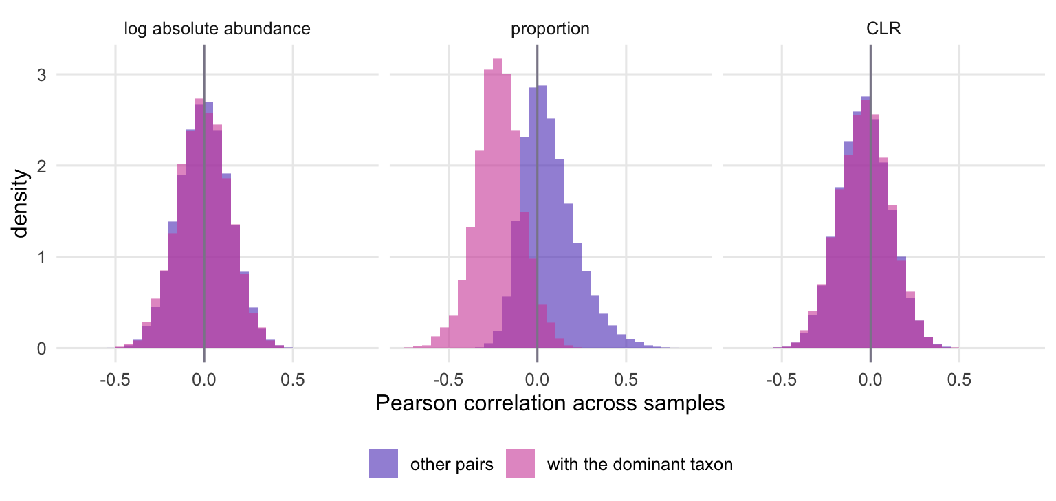
Figure 1: Pairwise correlations between taxa whose absolute abundances are independent, pooled over all simulated data sets. Pairs that include the dominant taxon are shown separately from all other pairs; each histogram is scaled to unit area.
The left panel is the truth: correlations of the log absolute abundances scatter around zero (mean -0.001), and 5.2% of pairs reach , as they should. The middle panel is what cor() on the proportions reports for the same samples. It is not one distribution but two. The pairs that include the dominant taxon are pushed down, to a median of -0.22, and 31% of them are “significant”. The other pairs are pushed slightly up, to a median of 0.05, and 9.7% of them pass . A network built from these correlations would put the dominant taxon at the centre of a star of negative edges, which looks like competition or exclusion and is purely arithmetic.
Spurious correlations of proportions are not always negative: here 63% of the pairs without the dominant taxon are positive. The identity only fixes the sum of each part’s covariances, and for a minor taxon the covariance with the dominant one more than covers it, leaving room for positive covariances with the other minor taxa.
A shared denominator
The positive side has an old explanation. The proportion of taxon is its abundance divided by the total, and the total is the same for every taxon in that sample. Two ratios with a common denominator are correlated even when their numerators are independent: when the denominator happens to be large, both ratios are small. Pearson (1897) described this “spurious correlation” for indices used in measuring organs, where one measurement is divided by another. When one taxon dominates, a large part of the total is that taxon, so every other proportion is roughly an independent abundance divided by the dominant one. They rise and fall together, and the dominant taxon moves against them.
Logs do not help, because still contains the shared total . With log proportions (a pseudocount of 0.5 for the few zeros) the other pairs have a median correlation of 0.15 and 19.1% of all pairs pass .
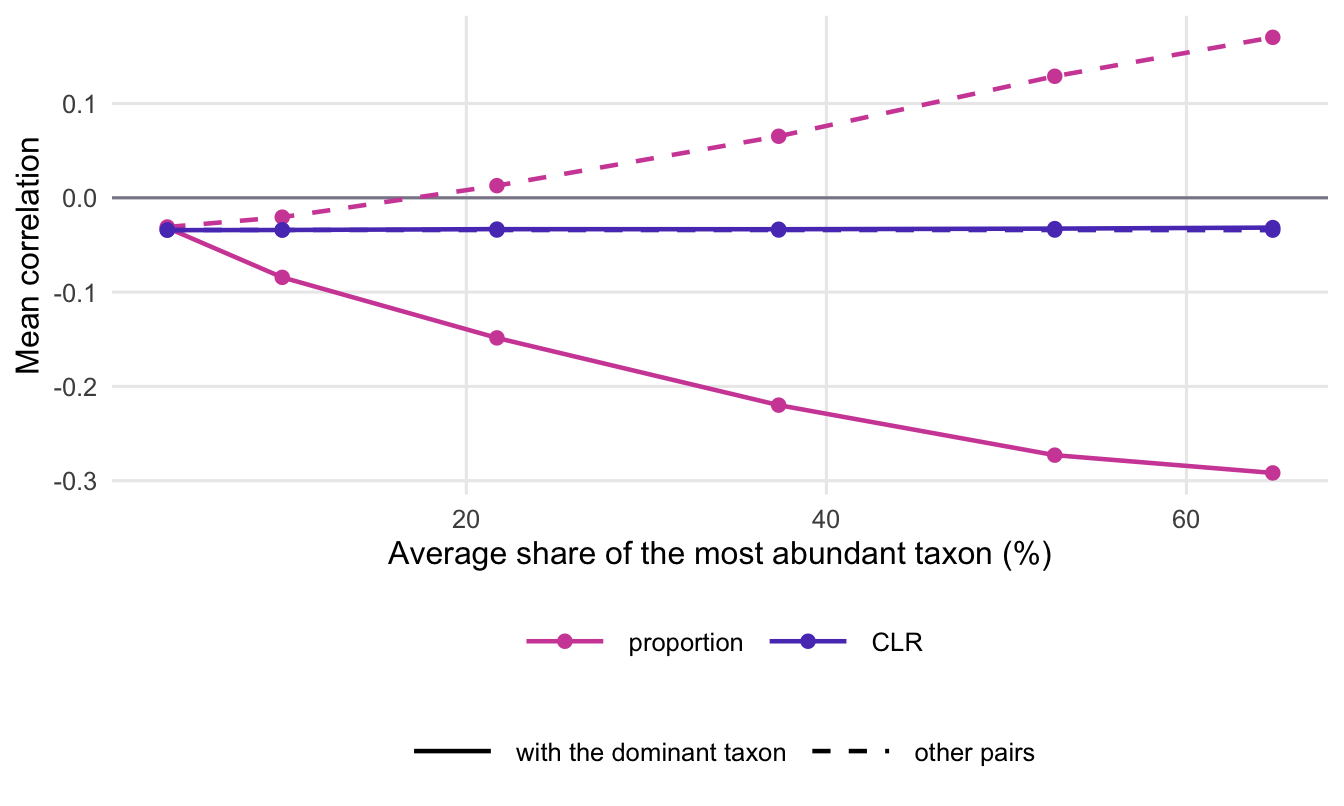
The strength of the effect depends on how dominant the largest taxon is. The next simulation keeps 30 independent taxa and makes the abundance curve steeper step by step, with 100 data sets per step.
dom_long <-rbind(data.frame(top = sweep_dom$top, r = sweep_dom$prop_dom, method ="proportion", pair ="with the dominant taxon"),data.frame(top = sweep_dom$top, r = sweep_dom$prop_oth, method ="proportion", pair ="other pairs"),data.frame(top = sweep_dom$top, r = sweep_dom$clr_dom, method ="CLR", pair ="with the dominant taxon"),data.frame(top = sweep_dom$top, r = sweep_dom$clr_oth, method ="CLR", pair ="other pairs"))dom_long$method <-factor(dom_long$method, levels =c("proportion", "CLR"))dom_long$pair <-factor(dom_long$pair, levels =c("with the dominant taxon", "other pairs"))ggplot(dom_long, aes(100* top, r, colour = method, linetype = pair)) +geom_hline(yintercept =0, colour = grey) +geom_line(linewidth =0.8) +geom_point(size =2) +scale_colour_manual(values =c(proportion = magenta, CLR = violet), name =NULL) +scale_linetype_manual(values =c("with the dominant taxon"="solid", "other pairs"="dashed"),name =NULL) +labs(x ="Average share of the most abundant taxon (%)", y ="Mean correlation") + theme_pc +theme(legend.box ="vertical", legend.key.width =unit(2.5, "lines"))
Figure 2: Mean correlation under independence as one taxon takes a larger share of the community, for proportions and for CLR values. Solid lines: pairs that include the most abundant taxon; dashed lines: all other pairs. The two CLR lines coincide.
With all taxa the same size (each about 3% of a sample), every pair of proportions has a mean correlation near -0.03. At the steepest curve the largest taxon holds 65%, its mean correlation with the others is -0.29, and the mean among the rest has risen to 0.17. The CLR lines barely move (-0.034 to -0.032), for the reason given next.
The centred log-ratio
The standard alternative comes from the log-ratio approach to compositional data (Aitchison 1982). The centred log-ratio (CLR) of a part is its log abundance minus the mean log abundance of all parts in that sample, which is the log of its ratio to the geometric mean. Two things follow. Dividing a sample by its total subtracts the same constant from every log, and the centring removes it, so the CLR values of proportions and of absolute abundances are identical. And every part contributes equally to the reference, whatever its size, so no single taxon can control it.
In the main simulation the CLR correlations have a mean of -0.034, the pairs with the dominant taxon have a median of -0.031, and 5.7% of all pairs reach . That is close to the 5.2% of the absolute abundances, and it is the right-hand panel of the first figure: the two groups of pairs now overlap.
The CLR needs the log of every count, and zeros have no log. The usual fix is to add a pseudocount, here 0.5, which has side effects of its own (see the post on pseudocounts and fold changes). In the main simulation zeros are rare, so the choice hardly matters. To see when it does, the next check uses a steeper abundance curve and shallower sequencing, and looks at the rarest taxa.
With 500 to 10,000 reads per sample, the 10 rarest taxa are zero in 30% of samples. On the absolute abundances, the CLR correlation among them averages -0.035. From the counts it averages -0.039 with a pseudocount of 0.1, -0.013 with 0.5 and 0.025 with 1. A pseudocount turns every zero into the same value, and zeros are more common in shallow samples, so the larger the pseudocount, the more the rare taxa share a dependence on sequencing depth. Their correlation with log depth averages -0.006, -0.125 and -0.204 for the three pseudocounts. The shift is small here, but the choice changes the answer.
What the CLR cannot fix
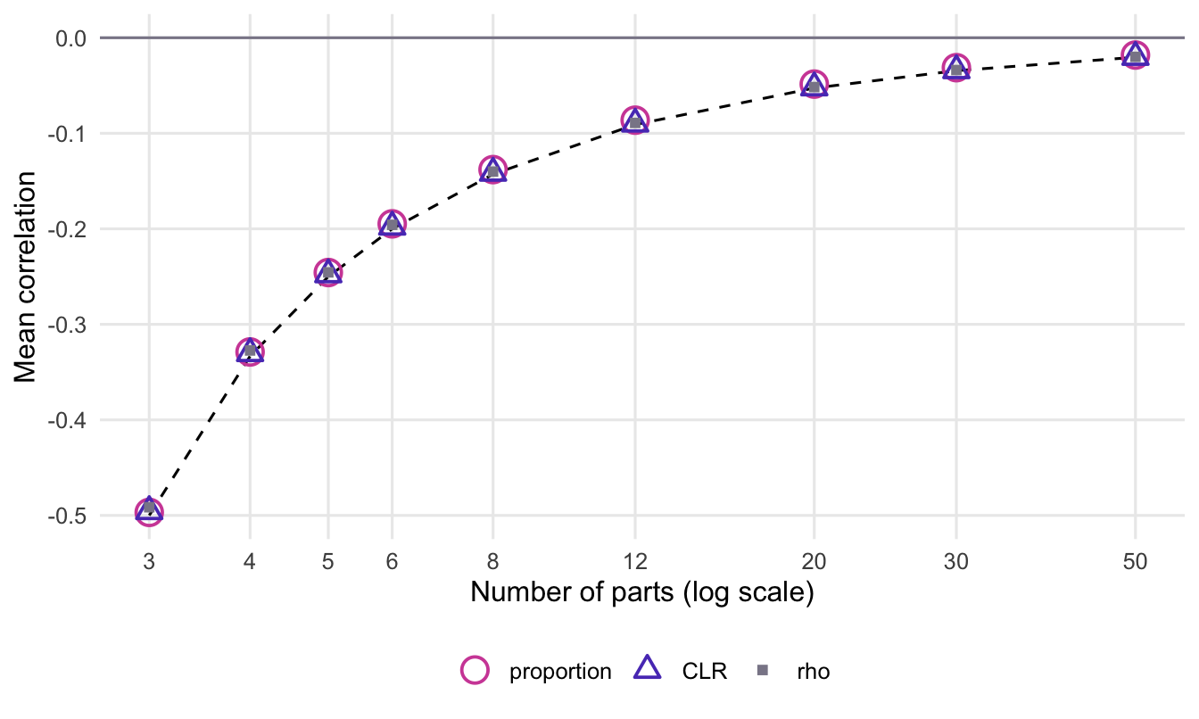
The CLR values of a sample also add up to zero, so the identity from the start applies to them too. With independent parts of equal log-scale variance it gives an exact result: the correlation between any two CLR values is for parts. With 30 taxa that is -0.034, which is the mean found above. With many parts this is close enough to zero to ignore; with few parts it is not.
Figure 3: Mean correlation under independence against the number of parts in an evenly balanced composition. The dashed curve is minus one over the number of parts minus one.
The simulation uses evenly sized parts, so there is no dominant one, and all three measures land on the curve. A single-cell study that tracks 5 cell types gets a mean CLR correlation of -0.25 between cell types that are independent, and 43% of pairs pass with 50 samples. With 8 parts it is still 16%; with 3 parts, 96%. Only with a few dozen parts does the rate come down to about 5% (5.5% at 30). These rates depend on the number of samples: with fewer donors fewer pairs reach significance, but the mean correlation stays where it is.
No transformation of the proportions removes this, because the information is not in the data. If five cell types always make up the whole, an increase in one must be matched by a decrease somewhere else, and nothing computed from the shares can say whether that was a real loss of cells or only a smaller slice of the same total.
Proportionality
The CLR fixes the dominant-part problem but still gives a correlation, and correlation is the wrong question for relative data. Lovell et al. (2015) propose asking instead whether two parts are proportional: whether their ratio stays constant across samples. The natural measure is the variance of the log-ratio, . Because , the total cancels, and this variance is the same whether you compute it from absolute abundances, from proportions, or from any subset of the parts.
A log-ratio variance on its own has no fixed scale, so it is usually rescaled. Lovell et al. divide it by the variance of one of the two parts and call the result phi. The symmetric version used here, (rho), is the one implemented in the propr R package, computed on CLR values by default (Quinn et al. 2017). It divides the log-ratio variance by the sum of the two CLR variances and subtracts the result from 1:
which is the same as
It is 1 when the two parts are exactly proportional, 0 when the log-ratio varies as much as the two parts together, and it is Lin’s concordance correlation coefficient without the term for a difference in means, so a constant ratio other than 1 still scores 1. The rho() function in the setup code implements it; the check after the main simulation confirms that a pair with gets exactly 1 before and after closure and that the matrix form matches the definition.
Under independence rho behaves like the CLR correlation: a mean of -0.034 in the main simulation, and the same curve in the last figure. So rho is not a test of independence, and it does not rescue a five-part composition. What it adds over a CLR correlation is a narrower question. A correlation is 1 for any straight-line relation between two CLR columns; rho is 1 only when the slope is 1, which on the log scale means the two parts are proportional. In a second toy check, one part is the square of another () among 9 other parts: their CLR correlation is 0.98 and their rho is 0.72. Two taxa that rise together, one much more steeply than the other, get a high correlation and a lower rho.
Changing the set of parts
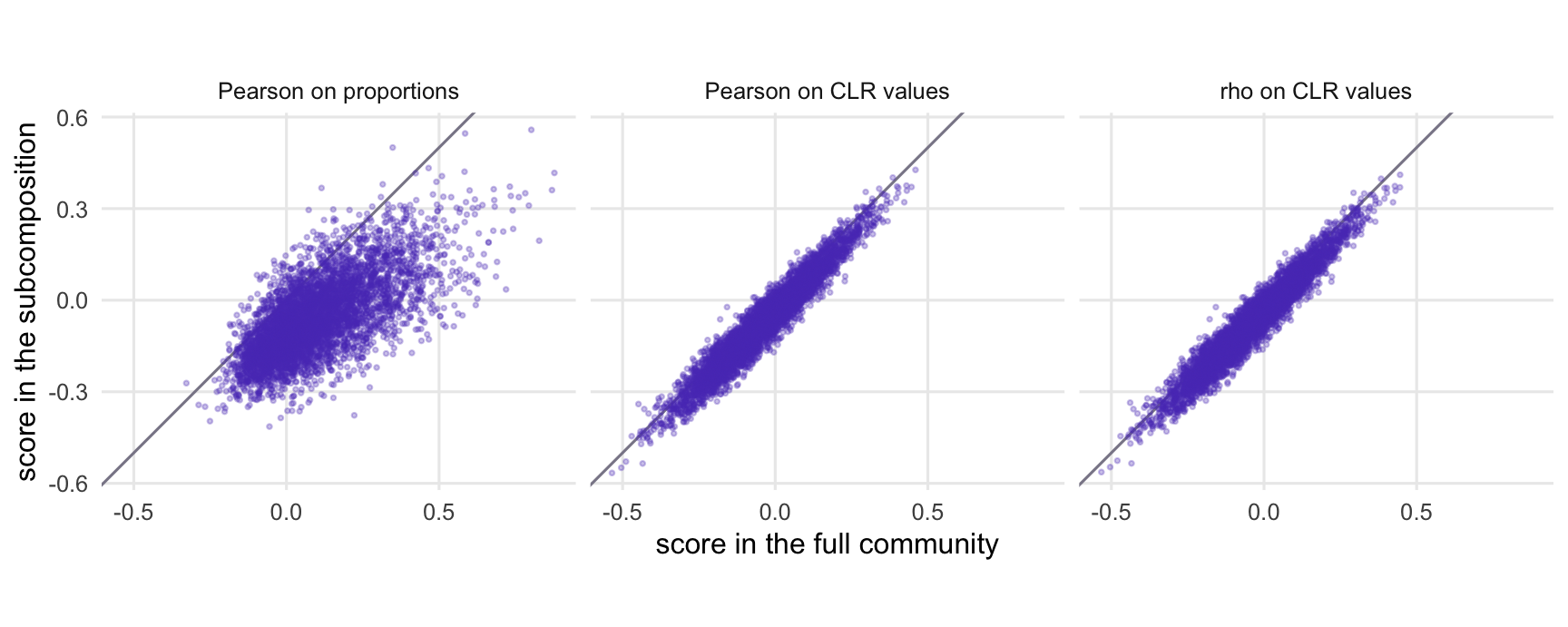
A correlation of proportions also depends on which other parts were measured. The next check scores the same pairs of the rarest half of the taxa twice: once in the full community, and once after the abundant taxa are dropped and the rest re-closed to 100%, as happens when a study reports only one phylum or excludes a contaminant.
sub_long <-rbind(data.frame(full = sub$cor_full, part = sub$cor_sub, score ="Pearson on proportions"),data.frame(full = sub$clr_full, part = sub$clr_sub, score ="Pearson on CLR values"),data.frame(full = sub$rho_full, part = sub$rho_sub, score ="rho on CLR values"))sub_long$score <-factor(sub_long$score, levels =unique(sub_long$score))ggplot(sub_long, aes(full, part)) +geom_abline(slope =1, intercept =0, colour = grey) +geom_point(size =0.6, alpha =0.3, colour = violet) +facet_wrap(~ score) +coord_equal() +labs(x ="score in the full community", y ="score in the subcomposition") + theme_pc
Figure 4: The same pairs of rare taxa scored in the full community (x axis) and after the abundant taxa are removed and the rest re-closed to 100% (y axis), with three scores. Points on the diagonal would mean the score does not depend on which other taxa were measured.
The correlation of proportions depends heavily on what else was measured. For the same pairs of taxa it averages 0.09 in the full community and -0.06 in the subcomposition, and the typical pair moves by 0.15 (median absolute change). Moving to log-ratios removes most of that. The CLR correlation moves by 0.04 and rho by 0.04; their averages go from -0.034 to -0.071 and from -0.033 to -0.070, the of 15 parts being -0.071. The two move the same small amount because both are scaled by CLR variances, and a CLR value depends on the geometric mean of whatever parts are present. The log-ratio variance itself does not move at all: the largest difference is 3e-15, which is floating-point rounding. If a result has to survive a change in which taxa were measured, the log-ratio variance of the pair is the quantity to report.
What to do in practice
Do not run cor() on proportions, percentages or their logs, and do not build co-occurrence networks from them. One dominant part against everything and the rest mildly positive looks like biology and is arithmetic.
With many parts, compute on CLR values. A pseudocount is needed only because of the zeros; say which one you used, and check that your conclusions hold with a second one. With CLR correlations or rho, report which parts went into the reference, because the numbers depend on it. For finding parts that move together, rho answers a question that relative data can actually support. It has no built-in test, and the propr paper picks its highly proportional pairs with an arbitrary cutoff. A cutoff can instead be calibrated by shuffling each taxon’s counts across samples, which destroys every pairing, and recording how high rho gets by chance:
x <- counts +0.5# samples in rows, taxa in columnsz <-log(x) -rowMeans(log(x)) # centred log-ratiov <-apply(z, 2, var)rho <-2*cov(z) /outer(v, v, "+") # proportionalitylr_var <-outer(v, v, "+") -2*cov(z) # var(log(x_i / x_j)) for every pair# permutation null for rho: shuffle each taxon independently, recomputenull_rho <-replicate(100, { xp <-apply(x, 2, sample) zp <-log(xp) -rowMeans(log(xp)); vp <-apply(zp, 2, var) r <-2*cov(zp) /outer(vp, vp, "+"); r[upper.tri(r)]})quantile(null_rho, 0.99) # rho this high arises by chance in 1% of pairs
With few parts, such as a handful of cell types, accept that the proportions are dependent and ask a question in ratio form instead: does the ratio of B cells to T cells change with treatment? That ratio is a single number per sample and can be tested like any other. If the question is really about absolute numbers (did this cell type expand, or did the others shrink?), it needs a measurement of the total: cells per microlitre from a counter or flow cytometry, a spike-in, or total bacterial load by qPCR. RNA-seq has the same problem when most genes change (see the post on CPM and TMM), and the same answer: the reference has to come from outside the shares.