Samples nested in donors: sums or duplicateCorrelation
experimental design
pseudoreplication
edgeR
limma
RNA-seq
Several RNA-seq samples per donor, donors nested in groups: why independent-sample tests inflate the FDR, and how donor sums or duplicateCorrelation handle it.
You have RNA-seq from 4 patients and 4 controls, with 3 biopsies from each person, and you want the genes that differ between patients and controls. That makes 24 samples. Can you analyse them as 24 replicates? No: for a comparison between groups of donors, the replicates are the donors, and there are 8 of them. In the simulation below, testing the 24 samples as independent with edgeR gave p < 0.05 for 17% (small donor effect) to 27% (large) of the genes with no true difference, where a valid test gives 5%, and 36% to 63% of the genes it called at a 5% false discovery rate (FDR) were false. Summing each donor’s counts into one profile and testing the 8 sums brought the first figure to between 4.9% and 6.1%.
Statisticians call the mistake pseudoreplication: treating repeated measurements of one unit as if they were independent units (Lazic 2010). This post measures what it costs, shows why the obvious repair (donor in the design formula) fails with a “not full rank” error, and compares the two standard fixes: one profile per donor, or limma’s duplicateCorrelation(). A shorter second part covers the case where the comparison is within donors and some donors are missing one of the two samples.
The setup
Each simulated experiment has 4 control donors and 4 disease donors, with 3 samples from each donor.
n_donor <-4# donors per groupn_per <-3# samples per donorsA <-data.frame(group =factor(rep(c("control", "disease"), each = n_donor * n_per)),donor =factor(sprintf("d%d", rep(seq_len(2* n_donor), each = n_per))))table(sA$donor, sA$group)
The counts are negative binomial, the usual model for RNA-seq read counts, for 1,000 genes. Each gene has a baseline level, and each donor shifts that level up or down at random: a normal effect on the log2 scale with a standard deviation (sd) of either 0.3 (a small donor effect) or 0.6 (a large one). The donor effect is drawn once per gene and donor, so all samples of a donor share it. On top of that, samples from the same donor differ from each other with the negative binomial’s own variation, which is relatively larger for weakly expressed genes, as in real data. Library sizes vary a little between samples.
Two assumptions matter. The donor effect is the only thing that makes a donor’s samples alike, and it is normal on the log scale with the same sd for every gene. Real donors also differ in genotype, age and sampling day, and some genes vary between people much more than others; the simulation keeps one sd so the mechanism stays visible.
In the “mixed” version of the experiment, 10% of the genes have a true log2 fold change of plus or minus 1 between disease and control; in the “global null” version, no gene does. Every analysis below runs on 4 replicate datasets of each version, at each of the two donor-effect sizes (except the slowest, which runs on the mixed version only; see the table below).
G <-1000# genes per simulated experimentprop_de <-0.1# share of genes with a true effectsim_genes <-function(prop_de, lfc) { mu0 <-exp(rnorm(G, log(150), 1.3)) # baseline mean count n_de <-round(prop_de * G)list(mu0 = mu0,phi =0.03+0.3/sqrt(mu0), # NB dispersion between samples of a donorlfc =c(sample(c(-1, 1) * lfc, n_de, TRUE), rep(0, G - n_de)))}sim_counts <-function(g, s, donor_sd, effect_col) { nd <-nlevels(s$donor) b <-matrix(rnorm(G * nd, 0, donor_sd), G, nd) # log2 donor effects, one per gene and donor lf <-outer(g$lfc, effect_col) + b[, as.integer(s$donor)] mu <- g$mu0 *2^lf *rep(runif(nrow(s), 0.7, 1.4), each = G) # library size differences m <-matrix(rnbinom(G *nrow(s), mu = mu, size =1/ g$phi), G, nrow(s))storage.mode(m) <-"integer" m}donor_sds <-c(0.3, 0.6) # small and large donor effect (log2 sd)lfc_a <-1# true log2 fold change, disease vs control
Why ~ donor + group is not full rank
The first repair most people try is to put donor in the design, as they would for a batch. It fails before any data are analysed:
# the disease column is the sum of the columns for the four disease donorssame_col <-all(X_nest[, "groupdisease"] ==rowSums(X_nest[, paste0("donord", (n_donor +1):(2* n_donor))]))same_col
[1] TRUE
set.seed(7)cts_demo <-sim_counts(sim_genes(0, 0), sA, donor_sds[1], rep(0, nrow(sA)))deseq_msg <-tryCatch(DESeqDataSetFromMatrix(cts_demo, sA, design =~ donor + group),error =function(e) conditionMessage(e))cat(strwrap(deseq_msg, 80), sep ="\n")
the model matrix is not full rank, so the model cannot be fit as specified.
One or more variables or interaction terms in the design formula are linear
combinations of the others and must be removed.

Please read the vignette section 'Model matrix not full rank':

vignette('DESeq2')
The design matrix has 9 columns but rank 8. Each donor belongs to one group only (donor is nested in group), so the “disease” column is the sum of the columns that mark the disease donors (the check above returns TRUE), and the group difference cannot be separated from the donor differences. DESeq2 stops when the data object is built; limma’s nonEstimable() names the coefficient that cannot be estimated. The DESeq2 vignette covers a related layout in its section on individuals nested within groups, where each individual is also measured under two conditions: a formula with both individual and group fails “because the effect for group is a linear combination of the individuals”, and its workaround tests group-specific condition effects within individuals. It offers no test of the group difference itself.
That leaves two routes for the group comparison. One is to reduce the data to one value per donor. The other is to model the donor as a random effect: instead of estimating a shift for every donor, estimate how much donors vary, and let that variation enter the standard error. DESeq2’s model (the “DESeq2 model” section of its vignette) is a generalised linear model whose coefficients are all fixed, so it has no random donor term. limma approximates one with duplicateCorrelation() (Smyth et al. 2005), which estimates the correlation between samples from the same donor and passes it to the linear model fit.
Five analyses
All five analyses below filter genes with edgeR’s filterByExpr() and normalise with normLibSizes(). The edgeR runs are the quasi-likelihood pipeline (Chen et al. 2016), with glmQLFit(robust = TRUE, legacy = FALSE); the limma runs use voom (Law et al. 2014), which turns counts into log-CPM values (log counts per million) with a precision weight for each value.
The two naive analyses fit ~ group to all 24 samples as if they were independent. The two collapsed analyses first add up each donor’s counts with edgeR::sumTechReps() (named for technical replicates, it simply sums the columns that share an ID) and fit ~ group to the 8 sums. The fifth analysis keeps all samples and follows the limma User’s Guide (its RNA-seq case study of Yoruba HapMap cell lines): voom, duplicateCorrelation() with block = donor, voom again with the block and the estimated correlation, duplicateCorrelation() again, then lmFit() with block and correlation.
prep <-function(cts, X) { y <-DGEList(cts) keep <-filterByExpr(y, X)list(y =normLibSizes(y[keep, , keep.lib.sizes =FALSE]), keep = keep)}full_p <-function(p, keep) { out <-rep(NA_real_, length(keep)); out[keep] <- p; out }edger_ql <-function(cts, X, coef) { pr <-prep(cts, X) fit <-glmQLFit(pr$y, X, robust =TRUE, legacy =FALSE)full_p(glmQLFTest(fit, coef = coef)$table$PValue, pr$keep)}voom_plain <-function(cts, X, coef) { pr <-prep(cts, X) fit <-eBayes(lmFit(voom(pr$y, X), X))full_p(fit$p.value[, coef], pr$keep)}# the limma user's guide recipe: voom, correlation, voom again with it, correlation againvoom_dupcor <-function(cts, X, coef, block) { pr <-prep(cts, X) v <-voom(pr$y, X) rho <-duplicateCorrelation(v, X, block = block)$consensus.correlation v <-voom(pr$y, X, block = block, correlation = rho) rho <-duplicateCorrelation(v, X, block = block)$consensus.correlation fit <-eBayes(lmFit(v, X, block = block, correlation = rho)) p <-full_p(fit$p.value[, coef], pr$keep)attr(p, "rho") <- rhoattr(p, "df") <- fit$df.residual[1] # residual df used by the t-tests p}run_a <-function(cts, s, dupcor =TRUE) { X <-model.matrix(~ group, s) sums <-sumTechReps(cts, s$donor) # one summed profile per donor sD <- s[!duplicated(s$donor), ] # sums come out in this donor order XD <-model.matrix(~ group, sD) out <-list("samples, edgeR"=edger_ql(cts, X, "groupdisease"),"samples, voom"=voom_plain(cts, X, "groupdisease"),"donor sums, edgeR"=edger_ql(sums, XD, "groupdisease"),"donor sums, voom"=voom_plain(sums, XD, "groupdisease"))if (dupcor) out[["voom + duplicateCorrelation"]] <-voom_dupcor(cts, X, "groupdisease", s$donor) out}expr_bins <-c(0, 50, 150, 500, 1e12) # baseline mean count binsscore <-function(p, de, mu0) { ok <-!is.na(p) called <- ok &p.adjust(p, "BH") <0.05# filtered genes count as not called nul <- ok &!de bin <-cut(mu0, expr_bins)data.frame(fpr =mean(p[nul] <0.05), # null genes with p < 0.05fpr01 =mean(p[nul] <0.01), # ... and with p < 0.01any_false =any(called &!de), # at least one false callcalls =sum(called),fdp =if (any(called)) mean(!de[called]) else0, # false discovery proportionpower =if (any(de)) mean(called[de]) elseNA_real_,bin =levels(bin),bin_hits =as.vector(tapply(p[nul] <0.05, bin[nul], sum)),bin_n =as.vector(table(bin[nul])))}
n_rep <-4resA <-list()set.seed(2026)for (r inseq_len(n_rep)) for (dsd in donor_sds) for (scen inc("global null", "mixed")) { g <-sim_genes(if (scen =="mixed") prop_de else0, lfc_a) cts <-sim_counts(g, sA, dsd, sA$group =="disease") P <-run_a(cts, sA, dupcor = scen =="mixed") # the slow fit on mixed data onlyfor (m innames(P)) resA[[length(resA) +1]] <-data.frame(rep = r, donor_sd = dsd, scenario = scen, method = m,score(P[[m]], g$lfc !=0, g$mu0),rho =if (is.null(attr(P[[m]], "rho"))) NA_real_elseattr(P[[m]], "rho"),df =if (is.null(attr(P[[m]], "df"))) NA_real_elseattr(P[[m]], "df"))}resA <-do.call(rbind, resA)
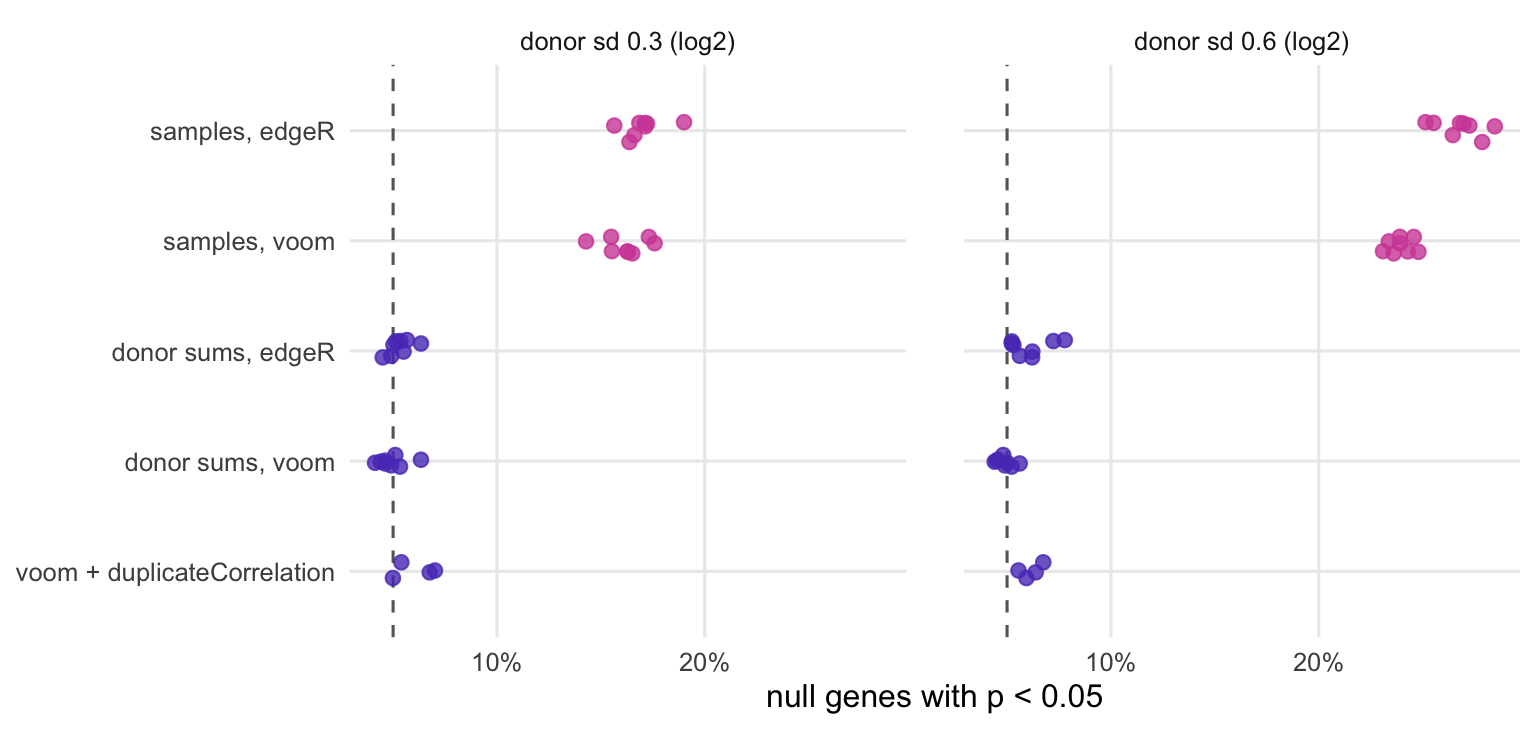
Figure 1: Share of genes without a true difference that reach p < 0.05, for each analysis and donor-effect size. Each dot is one simulated dataset (global null and mixed; duplicateCorrelation on the mixed datasets only); the dashed line marks the 5% a valid test gives.
With samples treated as independent, 17% (small donor effect) and 27% (large donor effect) of the null genes reach p < 0.05 with edgeR, and 16% and 24% with voom (Figure 1). In the mixed datasets, the share of false calls among the genes called at 5% FDR is 36% and 63% for edgeR. In the global-null datasets, where no gene has a true difference, naive edgeR called at least one gene in 8 of 8 datasets and naive voom in 8 of 8. The three donor-aware analyses stay close to the 5% line.
The damage follows from the correlation. When each donor contributes samples whose values are correlated with correlation , the variance of a group mean is larger than the naive formula assumes by the factor
With = 3 and the consensus correlations that duplicateCorrelation() estimated here (0.37 and 0.70 on average), the factor is 1.73 and 2.40. The naive test also believes it has 22 residual degrees of freedom, while the information about donor-to-donor variation comes from 8 donors. Both errors make the standard error too small, and both grow with the donor effect.
The table collects the numbers from this part. The two columns of null genes pool the global-null and mixed datasets; duplicateCorrelation(), the slow step of the whole post, was run on the mixed datasets only, hence its smaller number of datasets. The last three columns come from the mixed datasets: the average number of genes called at 5% FDR, the false discovery proportion (“FDP”, the share of called genes that have no true effect, whose average over datasets is the realised FDR) and the power.
The apparent power of the naive analyses (91% and 73% for edgeR, against 80% and 15% for edgeR on donor sums) is not information gained: it comes with the false calls. With 4 donors per group and the large donor effect, an honest analysis finds few of the true changes, and that is the real state of knowledge from 8 people. At that power, few genes are called in each dataset, so the realised FDR of the honest analyses rests on few calls and moves a lot between datasets.
duplicateCorrelation uses one correlation for all genes
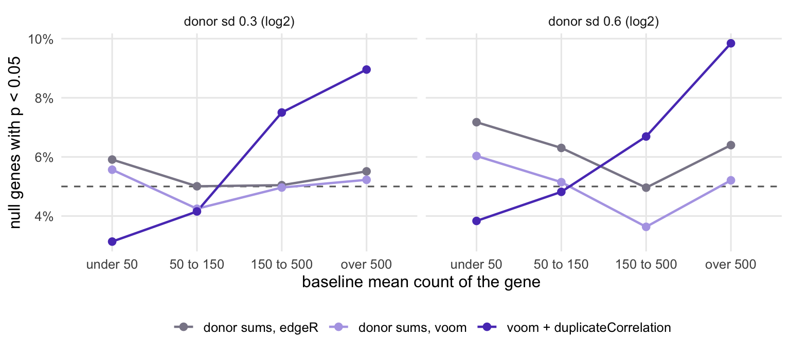
On average, duplicateCorrelation() gives 6.0% and 6.1% of null genes below p = 0.05, slightly above the nominal 5%. Voom on donor sums gives 4.9% and 4.9%. The overall figure hides a pattern, shown in Figure 2.
b3 <- binA[!grepl("^samples", binA$method), ]b3$bin <-factor(b3$bin, levels =levels(cut(1, expr_bins)),labels =c("under 50", "50 to 150", "150 to 500", "over 500"))b3$sd_lab <-factor(paste("donor sd", b3$donor_sd, "(log2)"))b3$method <-factor(b3$method, levels = meths[3:5])ggplot(b3, aes(bin, fpr, colour = method, group = method)) +geom_hline(yintercept =0.05, linetype ="dashed", colour ="grey40") +geom_line(linewidth =0.8) +geom_point(size =2.2) +facet_wrap(~ sd_lab) +scale_y_continuous(labels = pct_axis) +scale_colour_manual(values =c(grey, lilac, violet), name =NULL) +labs(x ="baseline mean count of the gene", y ="null genes with p < 0.05") + theme_pc
Figure 2: Share of null genes with p < 0.05, split by the gene’s baseline mean count, for the three donor-aware analyses. Pooled over the datasets each analysis was run on; the dashed line marks 5%.
For the most highly expressed genes (baseline mean above 500 counts), 9% and 10% of null genes reach p < 0.05 with duplicateCorrelation(); for the weakest (below 50), 3% and 4%. The reason is in the name of the output: consensus.correlation is a single number for all genes, a trimmed mean of the gene-wise estimates on the atanh scale (its help page). But the true within-donor correlation differs between genes. The donor effect is the same for every gene here, while the sample-to-sample noise of a weakly expressed gene is larger, so a weak gene’s samples resemble each other less. A rough calculation (the delta method, on the log2 scale) puts the correlation at about 0.27 for a gene with a mean of 30 counts and 0.52 for one with 1,000 counts under the small donor effect, and at 0.59 and 0.81 under the large one. The consensus sits in between, so it is too low for highly expressed genes (standard errors too small, too many small p-values) and too high for weakly expressed ones. In real data, genes also differ in how much they vary between people, which spreads the true correlations further.
A second effect is the degrees of freedom. lmFit() with a correlation treats the correlation as known and uses 22 residual degrees of freedom, as for a fit to 24 independent samples, although the group comparison rests on 8 donors. With few donors per group, that leans towards small p-values as well. Donor sums avoid both problems: each gene gets its own between-donor variance, estimated from the donors themselves. edgeR on the sums is close to 5% at the small donor effect (5.3%) and a little above it at the large one (6.1%). One likely reason: the donor effects here are normal on the log scale, which matches voom’s log-scale linear model and fits the count model only approximately.
In power, the collapsed analyses and duplicateCorrelation() are close: 80%, 80% and 79% (voom on sums, edgeR on sums, duplicateCorrelation) at the small donor effect, and 15%, 15% and 17% at the large one. With the same number of samples per donor, the sum loses very little: a between-donor comparison can only use what the donor means carry. For designs where one correlation for all genes is too crude, Hoffman and Roussos (2021) describe dream() in the variancePartition package, a differential expression method for repeated-measures designs; it is not run here.
Within-donor comparisons with missing partners
The balance tips the other way when the question is inside donors: treated against untreated samples from the same people, with some donors missing one of the two. Here there are 6 complete pairs, and 4 donors with a single sample (2 untreated, 2 treated). 10% of genes have a true log2 fold change of plus or minus 0.75 within donors.
Now ~ donor + cond is full rank, and donor as a fixed block (a coefficient per donor) is the standard analysis in all three packages: the treatment effect is estimated from differences within donors, and a donor with a single sample is fitted exactly by its own coefficient, so it adds nothing to the treatment estimate. duplicateCorrelation() with ~ cond can use those single samples too, because it treats the donor effect as random and so also compares untreated and treated samples from different donors, weighted by how much donors vary. This is the use in the example on duplicateCorrelation()’s help page, a paired experiment with incomplete blocks.
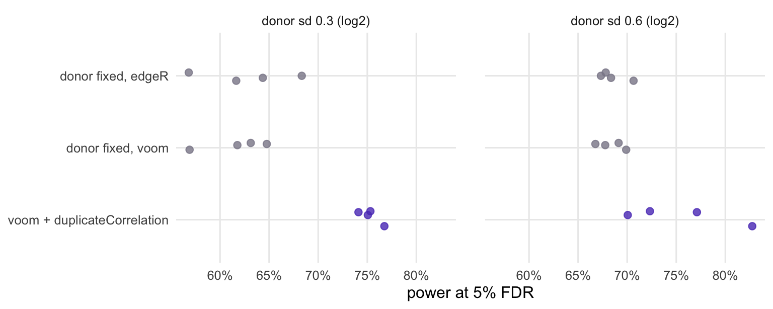
Figure 3: Power at 5% FDR for the within-donor treatment effect, with some donors missing one sample. Each dot is one simulated dataset.
duplicateCorrelation() finds 75% and 76% of the true changes (small and large donor effect), against 62% and 68% for voom with donor as a fixed block and 63% and 68% for edgeR with donor as a fixed block (Figure 3). The fixed-block numbers differ between the two donor-effect sizes only by chance, because the donor effect cancels within donors. Two things contribute to the gain: the single samples, and degrees of freedom (the fixed-block model has 5 residual degrees of freedom, the correlation model 14; this is the same optimistic count as in the first part, since the correlation is treated as known).
The price is error control. With duplicateCorrelation(), 5.7% and 5.5% of null genes reach p < 0.05, against 5.3% and 4.9% for voom with the fixed block. The realised FDR of duplicateCorrelation() is 3.2% at the small donor effect and 7.7% at the large one, against 3.8% and 4.7% for voom and 4.6% and 4.4% for edgeR with the fixed block. These are averages over 4 datasets per setting, so each is rough. With complete pairs only, the fixed block is the simpler choice and needs no assumption about how donors vary.
What to do in practice
Before any model, count donors, not samples: table(samples$donor, samples$group) tells you how many independent units each group has. If every donor sits in one group, the group comparison is a comparison of donors.
For a between-group question, the simplest honest analysis collapses to one profile per donor and runs the usual pipeline on it:
sums <- edgeR::sumTechReps(counts, ID = samples$donor) # columns in order of first appearancedonors <- samples[!duplicated(samples$donor), ]y <- edgeR::DGEList(sums)X <-model.matrix(~ group, donors)keep <- edgeR::filterByExpr(y, X)y <- edgeR::normLibSizes(y[keep, , keep.lib.sizes =FALSE])fit <- edgeR::glmQLFit(y, X, robust =TRUE, legacy =FALSE)edgeR::topTags(edgeR::glmQLFTest(fit, coef =2))
The same sums can go into DESeqDataSetFromMatrix() with ~ group (DESeq2 was not part of the comparison above). If you need the individual samples in the model (a within-donor factor as well, or unequal numbers of samples per donor), use the limma recipe with the donor as block:
edgeR’s voomLmFit() (in edgeR since version 3.30.2, according to its NEWS file) runs the same two rounds of weights and correlation when given block, and also accounts for degrees of freedom lost to exact zero counts. Whichever you use, remember that the consensus correlation is an average: genes whose own within-donor correlation is above it get p-values that are too small. In this simulation those were the highly expressed genes; in real data, genes that vary a lot between people are candidates too. Check the p-value histogram of the result (see how to read a p-value histogram).
For a within-donor question with complete pairs, put donor in the design as a fixed block (~ donor + condition). With donors missing one of the conditions, duplicateCorrelation() uses the incomplete donors as well and gains power, at the cost of the one-correlation assumption and, in this simulation, a realised FDR above the nominal 5% when donors differ a lot.
The same logic applies to single-cell data, where cells from one donor are the extreme case of samples nested in donors; the pseudobulk post measures it there.