Pseudobulk for single-cell DE: should you sum or average counts, and do donors with few cells need a floor? A simulation with edgeR, DESeq2 and limma answers.
Author
Pseudocount
Published
16 November 2026
Setup: packages and helper functions
suppressPackageStartupMessages({library(edgeR)library(DESeq2)library(limma)library(ggplot2)})stopifnot(packageVersion("edgeR") >="4.0.0", packageVersion("DESeq2") >="1.40.0",packageVersion("limma") >="3.58.0", packageVersion("ggplot2") >="3.4.0")knitr::read_chunk("pseudobulk_sim.R") # the simulation and analysis functions belowalpha <-0.05# significance and FDR thresholdviolet <-"#5a3fc0"; magenta <-"#d14fa6"; grey <-"#8a8799"fmt_pct <-function(x, d =0) sprintf(paste0("%.", d, "f%%"), 100* x)fmt_int <-function(x) format(round(x), big.mark =",", trim =TRUE)fmt_num <-function(x, d =2) sprintf(paste0("%.", d, "f"), x)theme_set(theme_minimal(base_size =12) +theme(panel.grid.minor =element_blank(),plot.background =element_rect(fill ="white", colour ="white"),strip.text =element_text(face ="bold")))
The post on cells as replicates ended with a recipe: add up the raw counts of each donor’s cells within a cell type (a pseudobulk), then run a bulk RNA-seq method on one column per donor. The questions that follow are practical. Should the counts be summed or averaged? Should the sum be divided by the number of cells, so that a donor with 800 cells does not swamp a donor with 12? And should the donor with 12 cells be in the analysis at all?
Sum, do not divide, and think twice before dropping the small donor. In 60 simulated experiments with 4 donors per group, summed counts analysed with edgeR found 39% of the truly changed genes at an FDR of 5%. Dividing each sum by its number of cells, rounding, and running DESeq2 found 0.03% (3 significant genes in all 60 experiments together). Averaging log-normalised values per donor and running limma-trend found 25% and shrank the fold changes by about 35%. Dropping the donors with fewer than 50 cells lowered the edgeR figure by 13 percentage points.
The setup
# One cell type, one pseudobulk per donor. Counts per cell are negative binomial.sim_cells <-function(n_cells =c(800, 400, 150, 60, 300, 100, 30, 12),group =rep(c("ctrl", "trt"), each =4),n_genes =2000, de_frac =0.1, donor_sd =0.3,phi =0.3, capture_sd =0.3, lfc_range =c(0.5, 1.5)) { n_donor <-length(n_cells) donor <-rep(seq_len(n_donor), n_cells) # donor of each cell mu <-exp(rnorm(n_genes, log(0.5), 1)) # baseline mean UMI per cell is_de <-seq_len(n_genes) <=round(de_frac * n_genes) # the first genes truly change lfc2 <-ifelse(is_de, sample(c(-1, 1), n_genes, replace =TRUE) *runif(n_genes, lfc_range[1], lfc_range[2]), 0) # true log2 fold change b <-matrix(rnorm(n_genes * n_donor, 0, donor_sd), n_genes, n_donor) # donor effects trt <-as.numeric(group =="trt") donor_mean <- mu *exp(b +outer(lfc2 *log(2), trt)) # genes x donors s <-exp(rnorm(length(donor), -capture_sd^2/2, capture_sd)) # capture per cell m <- donor_mean[, donor] *rep(s, each = n_genes) counts <-matrix(rnbinom(length(m), mu = m, size =1/ phi), n_genes)list(counts = counts, donor = donor, group =factor(group), n_cells = n_cells,is_de = is_de, lfc2 = lfc2)}
aggregate_donors <-function(sim) { counts <- sim$counts sums <-t(rowsum(t(counts), sim$donor)) # summed raw counts means <-sweep(sums, 2, sim$n_cells, "/") # the same, divided by cells lognorm <-log1p(sweep(counts, 2, colSums(counts), "/") *1e4) # LogNormalize mean_log <-t(rowsum(t(lognorm), sim$donor)) /rep(sim$n_cells, each =nrow(counts))list(sums = sums, means = means, mean_log = mean_log)}
Each simulated experiment is one cell type from 8 donors, half control and half treated, with 2,000 genes. The number of cells per donor is deliberately uneven and deliberately unbalanced between the groups: the control donors have 800, 400, 150, 60 cells and the treated donors 300, 100, 30, 12, so 1,410 control cells face 442 treated ones. Real data look like this when a treatment depletes the cell type, or when some samples dissociated badly. The imbalance matters for two reasons: the lower cell floors tried below remove treated donors only (the highest also removes one control donor), and the treated pseudobulks have smaller libraries, so the normalisation has to do real work.
Counts per cell are negative binomial. Each gene has a baseline level, each cell a capture efficiency, and each donor’s level of each gene is shifted up or down at random, with a standard deviation of 0.3 on the natural log scale (the same donor effect as in the earlier post). The donor effect is the assumption that matters most here, and the last section varies it. The first 200 genes change with treatment, by a log2 fold change between 0.5 and 1.5 in either direction; the others are null, so any of them called significant is a false positive.
Three ways to build a pseudobulk
aggregate_donors() above builds the three candidates from the same cells. The first is the sum of the raw counts per donor. That gives an ordinary count matrix, one column per donor, which is what edgeR and DESeq2 are built to model. The donor with 800 cells has a far larger library than the donor with 12, and that is expected: both packages compare each gene with the size of the library it came from.
The size factors DESeq2 estimates from the sums follow the number of cells: the largest is 70 times the smallest, where the cell numbers differ 67-fold. So “divide by the number of cells” is already happening, inside the model, where it costs nothing.
The second candidate does the division by hand: the sum divided by the number of cells, which is the mean count per cell. These values are not integers, and DESeq2 refuses them:
The usual next step is to round them, and that is a misuse. The DESeq2 vignette asks for un-normalised counts, because only the count values let the model assess the measurement precision, and it says that normalised values such as counts scaled by library size should not be used as input. Dividing by the number of cells is the same kind of scaling. The result is on the per-cell scale, where 72% of the tested genes here average less than one UMI, so rounding turns 50% of the values into zeros.
The third candidate works on the log scale: Seurat-style log-normalisation of each cell (counts scaled to a fixed total per cell, plus one, natural log), averaged over each donor’s cells, then limma with an intensity-dependent variance trend (limma-trend). This is a legitimate route, since limma is built for log-expression values, but it throws information away. The mean of logs is not the log of a mean, and for genes with few UMIs per cell the “+1” inside the log flattens differences (the pseudocount post shows the same effect on fold changes). It is also outside the conditions the limma User’s Guide gives for limma-trend, which usually works well when the largest library is no more than about three times the smallest. Here the number of cells behind each mean plays the role of library size, and it ranges from 12 to 800.
In Seurat, AggregateExpression() is the first route: it always adds up the counts layer, and with the default return.seurat = FALSE it returns the sums without normalising them. AverageExpression() is closest to the second. By default it takes the log-normalised data layer, undoes the log (expm1), averages, and returns the averages on that normalised, non-log scale, so its output is not a count; it also prints a message (once per session) recommending AggregateExpression() for pseudobulk analysis. (Seurat 5.0.1 and 5.5.1 source.)
The analysis code for all routes is below. The summed counts go through the edgeR quasi-likelihood recipe (Chen et al. 2016; Chen et al. 2025 for the edgeR 4 method), the standard DESeq2 workflow (Love et al. 2014), limma-voom (Law et al. 2014) and voom with sample quality weights (Liu et al. 2015). legacy = FALSE is set explicitly because its default differs between edgeR releases (TRUE in 4.0.16, FALSE in 4.8.2), voom’s lowess span is fixed at its old default because limma 3.66 added an adaptive span that 3.58 lacks, and alpha in DESeq2’s results() is set to the FDR threshold, as its documentation asks when the threshold is not 0.1. Every method tests the genes kept by filterByExpr() on the sums (the floor routes filter again after dropping donors, as a user would).
run_methods <-function(sim, agg, floors =c(20, 50, 100), deseq =TRUE,mean_log =TRUE, alpha =0.05) { g <- sim$group; n <- sim$n_cells; sums <- agg$sums design <-model.matrix(~ g) keep <-filterByExpr(DGEList(sums, group = g), design) # one gene set for all methods fill <-function(x, rows = keep) {z <-rep(NA_real_, nrow(sums)); z[rows] <- x; z} out <-list()# summed counts + edgeR quasi-likelihood; optionally only donors with >= floor cells edger_ql <-function(cols) { gg <-droplevels(g[cols]); d <-model.matrix(~ gg) y <-DGEList(sums[, cols], group = gg) k <-filterByExpr(y, d) y <-normLibSizes(y[k, , keep.lib.sizes =FALSE]) fit <-glmQLFit(y, d, robust =TRUE, legacy =FALSE) tt <-glmQLFTest(fit, coef =2)$tablelist(p =fill(tt$PValue, k), lfc =fill(tt$logFC, k)) } out$sum_edger <-edger_ql(seq_along(n))for (f in floors) out[[paste0("floor", f)]] <-edger_ql(which(n >= f))# summed counts + voom, and + voomWithQualityWeights. limma 3.66 added# adaptive.span (default TRUE); fixing it to FALSE gives span = 0.5 in every version. y <-normLibSizes(DGEList(sums, group = g)[keep, , keep.lib.sizes =FALSE]) span_arg <-if ("adaptive.span"%in%names(formals(voom))) list(adaptive.span =FALSE) v <-do.call(voom, c(list(y, design, span =0.5), span_arg)) fit <-eBayes(lmFit(v, design)) out$sum_voom <-list(p =fill(fit$p.value[, 2]), lfc =fill(fit$coefficients[, 2])) vq <-do.call(voomWithQualityWeights, c(list(y, design, span =0.5), span_arg)) fit <-eBayes(lmFit(vq, design)) out$sum_voomqw <-list(p =fill(fit$p.value[, 2]), lfc =fill(fit$coefficients[, 2]),weights = vq$targets$sample.weights)if (deseq) {# summed counts + DESeq2 standard workflow cnt <-round(sums[keep, ]); storage.mode(cnt) <-"integer"# sums are whole numbers dds <-DESeq(DESeqDataSetFromMatrix(cnt, data.frame(g = g), ~ g), quiet =TRUE) r <-results(dds, name ="g_trt_vs_ctrl", alpha = alpha) out$sum_deseq2 <-list(p =fill(r$pvalue), lfc =fill(r$log2FoldChange),padj =fill(r$padj))# MISUSE: counts divided by the number of cells, rounded to integers, into DESeq2.# The default dispersion fit often breaks down on these values, so fitType = "mean"# is used; if even that stops, DESeq2's own advice in the error message is followed# (gene-wise dispersion estimates, then the Wald test). cnt <-round(agg$means[keep, ]); storage.mode(cnt) <-"integer" dds <-DESeqDataSetFromMatrix(cnt, data.frame(g = g), ~ g) route <-"mean fit" dds <-tryCatch(DESeq(dds, fitType ="mean", quiet =TRUE), error =function(e) { route <<-"gene-wise" dds <-estimateDispersionsGeneEst(estimateSizeFactors(dds))dispersions(dds) <-mcols(dds)$dispGeneEstnbinomWaldTest(dds, quiet =TRUE) }) r <-results(dds, name ="g_trt_vs_ctrl", alpha = alpha) out$mean_deseq2 <-list(p =fill(r$pvalue), lfc =fill(r$log2FoldChange),padj =fill(r$padj), zero_share =mean(cnt ==0),route = route) }if (mean_log) {# mean of log-normalised values per donor + limma-trend (natural log -> log2) fit <-eBayes(lmFit(agg$mean_log[keep, ], design), trend =TRUE) out$meanlog_trend <-list(p =fill(fit$p.value[, 2]),lfc =fill(fit$coefficients[, 2] /log(2))) }attr(out, "keep") <- keep out}
What each route finds
The table has the averages over 60 simulated experiments, computed by the script at the end of the post with edgeR 4.8.2, DESeq2 1.50.2 and limma 3.66.0. FPR is the share of null genes with p below 0.05. Calls is the average number of genes significant at an FDR of 5%, observed FDR the share of those calls that are null (zero when there are no calls), and power the share of the 200 changed genes that were called. The last two columns compare the estimated log2 fold changes of the changed genes with the truth: the root mean squared error, and the slope of estimate on truth (below 1 means the estimates are shrunk).
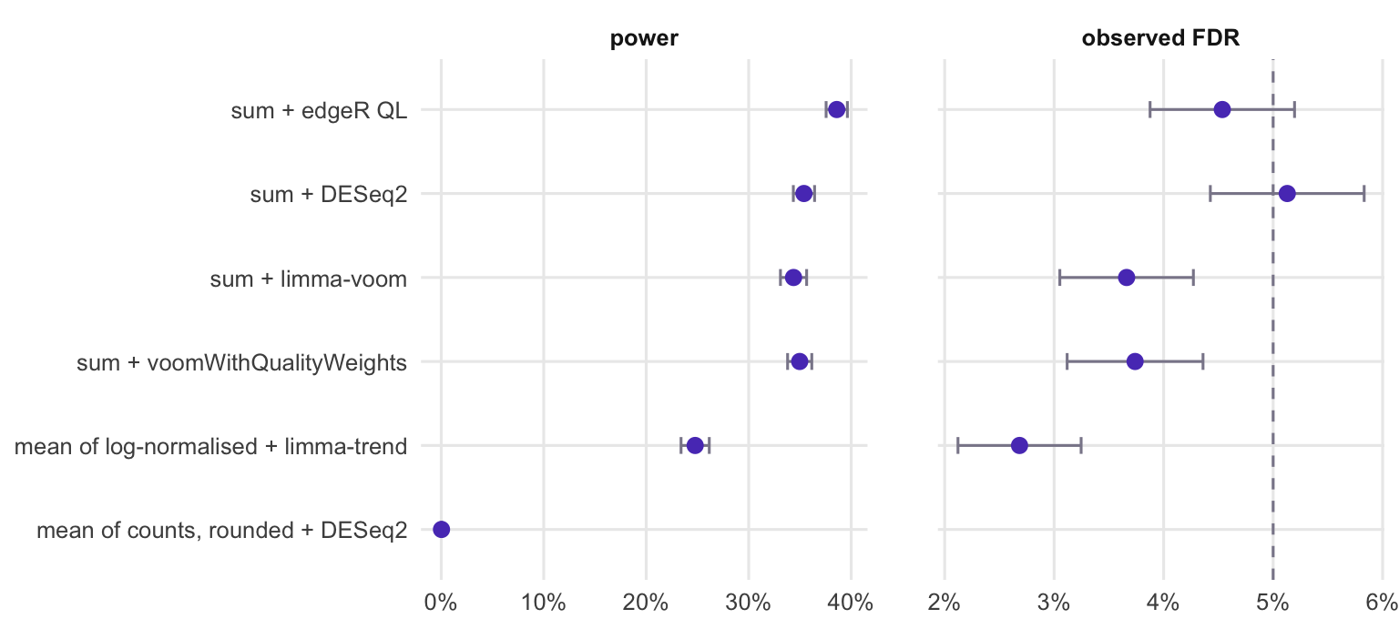
The four routes on summed counts do what their documentation promises. Their observed FDR ranged from 3.7% to 5.1% and their false positive rate from 4.9% to 5.4%, close to the nominal 5%. edgeR found 38.6% of the changed genes, DESeq2 35.4% and limma-voom 34.4%. None of them was told how many cells each donor had; the library sizes carried that information.
Dividing by the number of cells and rounding destroyed the analysis. DESeq2 on the rounded means found 0.03% of the changed genes, which is 3 significant genes over all 60 experiments. The mean of log-normalised values with limma-trend kept its error rates (observed FDR 2.7%) but found 24.8% of the changed genes, and apart from the rounded-mean route its fold changes had the largest error. Figure 1 puts power and observed FDR side by side.
Figure 1: Power and observed false discovery rate at the FDR threshold used in the text, averaged over the simulated data sets. Bars show two Monte Carlo standard errors; the dashed line in the right panel is the promised FDR. The rounded-mean route has no FDR point because it made almost no calls.
Why dividing by the number of cells fails
The rounded means fail for a reason that goes beyond rounding error. A negative binomial model reads each value as a number of molecules, with the Poisson noise that so many molecules carry. A mean over hundreds of cells is far more precise than a single count of the same size: for a mean over cells, the Poisson noise is smaller by a factor of . The model therefore expects more noise than the values show, the gene-wise dispersion estimates collapse towards zero, and DESeq2’s fit of the dispersion trend often breaks down. Over the 60 experiments, the default fit ran without a fallback or an error in 22, fell back to a local regression (with a message) in 21 and stopped with an error in 17. The analysis above therefore uses fitType = "mean", and where even that stopped (6 experiments) it follows the advice printed in DESeq2’s own error message. Whichever way it runs, the test sees small differences against inflated noise and calls almost nothing: its false positive rate was 0.03% against the nominal 5%, so here it is not unsafe, only blind.
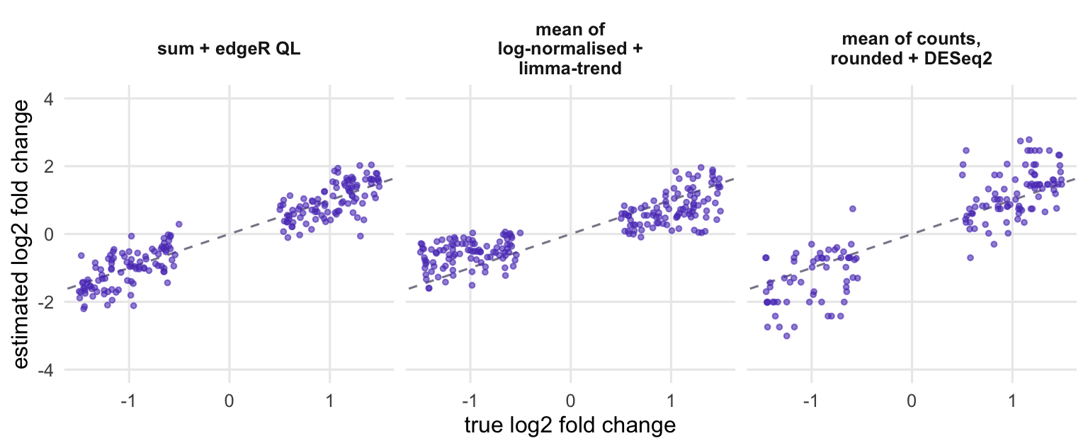
Rounding adds its own damage: 49% of the rounded values were zero, for 24% of the changed genes all of them were (so DESeq2 gives no fold change), and the remaining estimates had an error of 0.65 on the log2 scale against 0.38 for the sums (Figure 2, right).
The mean of log-normalised values fails more gently. Its test is calibrated, but the fold changes it reports are shrunk: a fitted slope of 0.65 against the true log2 fold changes (Figure 2, middle).
out <-run_methods(sim, agg)demo_route <- out$mean_deseq2$route
Figure 2: Estimated against true log2 fold change for the truly changed genes in one simulated data set. The diagonal is perfect estimation.
Should a small donor count as much as a large one?
In the summed-count analysis it does not count the same, and no extra rule is needed to make it so. A count model knows that a gene with a handful of reads in a small library is measured less precisely than the same gene with hundreds of reads in a large one, and edgeR, DESeq2 and voom all weight each observation by its expected precision. What the model does not know is that a small pseudobulk also carries more cell-to-cell variation. Each cell varies around its donor’s level by more than Poisson noise, and summing cells shrinks the contribution of that extra variation to the dispersion by a factor of . For a pseudobulk of cells, the negative binomial dispersion is approximately
where is the part due to donors differing (with the donor standard deviation on the natural log scale) and is the cell-level dispersion, 0.3 in this simulation (a small correction for differences in capture between cells is left out). edgeR and DESeq2 estimate one dispersion per gene, shared by all samples, so a small pseudobulk is noisier than the model assumes by the second term. The code below measures the dispersion directly on simulated donors.
levels_n <-c(10, 25, 50, 100, 200, 400, 800); reps <-10disp_sd <-c(0.1, donor_sd_main)disp <-do.call(rbind, lapply(disp_sd, function(sd_i) {set.seed(3) s <-sim_cells(n_cells =rep(levels_n, each = reps), group =rep("ctrl", reps *7),n_genes =1000, de_frac =0, donor_sd = sd_i) sums <-t(rowsum(t(s$counts), s$donor))do.call(rbind, lapply(levels_n, function(n) { cols <-which(s$n_cells == n) # 10 donors with n cells each y <-DGEList(sums[, cols]) y <-normLibSizes(y[filterByExpr(y, group =rep(1, reps)), , keep.lib.sizes =FALSE]) d <-estimateDisp(y, design =matrix(1, reps, 1))data.frame(donor_sd = sd_i, cells = n, dispersion = d$common.dispersion) }))}))disp$donor_part <-exp(disp$donor_sd^2) -1disp$approx <- disp$donor_part + phi_cell *exp(formals(sim_cells)$capture_sd^2) / disp$cellsdsp <-function(sd_i, n) disp$dispersion[disp$donor_sd == sd_i & disp$cells == n]n_lo <-min(levels_n); n_hi <-max(levels_n)ratio_hi_sd <-dsp(disp_sd[2], n_lo) /dsp(disp_sd[2], n_hi)ratio_lo_sd <-dsp(disp_sd[1], n_lo) /dsp(disp_sd[1], n_hi)breakeven <- phi_cell / (exp(disp_sd^2) -1) # cells at which the two terms are equal
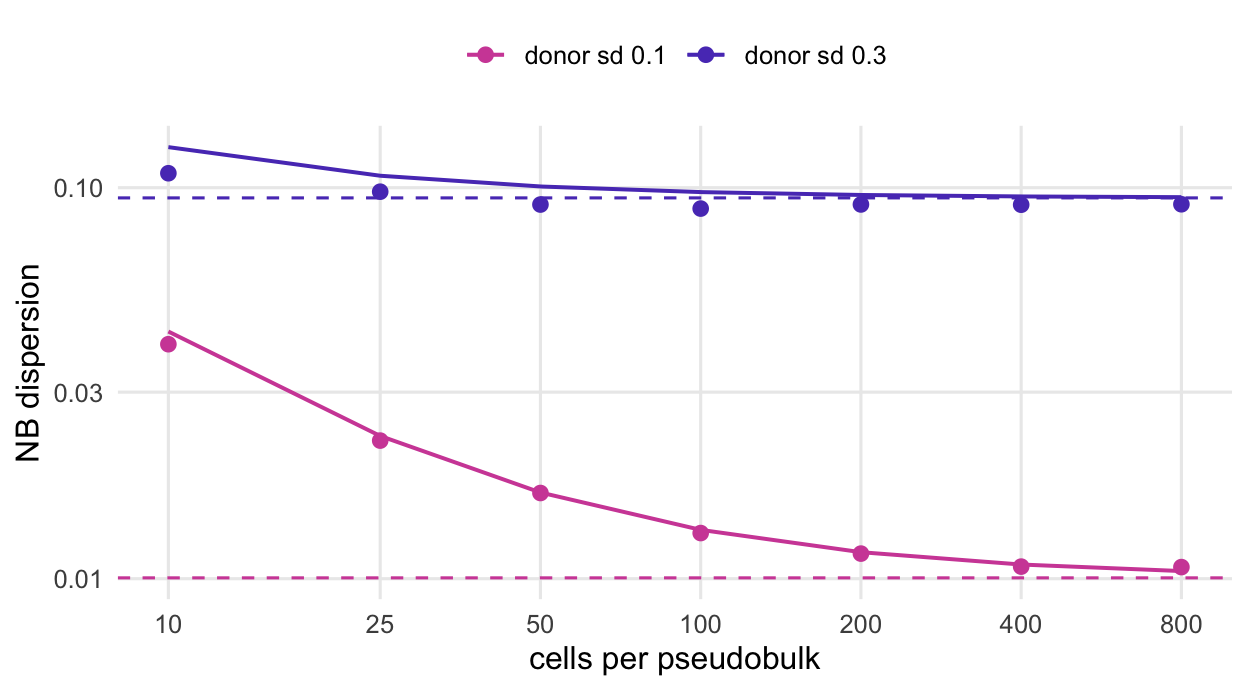
Figure 3: Dispersion of summed-count pseudobulks against the number of cells behind each one, for two sizes of donor-to-donor variation. Points: edgeR common dispersion from simulated donors that all have the same number of cells. Solid lines: the approximation in the text, including the small capture correction. Dashed lines: the donor part alone.
Figure 3 shows how much that second term matters. With the donor standard deviation of the main simulation, 0.3, the dispersion at 10 cells was only 1.2 times its value at 800 cells: the differences between donors swamp the extra cell-level noise, and by the formula the two terms are equal at about 3 cells. With a standard deviation of 0.1, for donors that are much more alike, the dispersion at 10 cells was 3.7 times its value at 800, and the break-even point moves to about 30 cells.
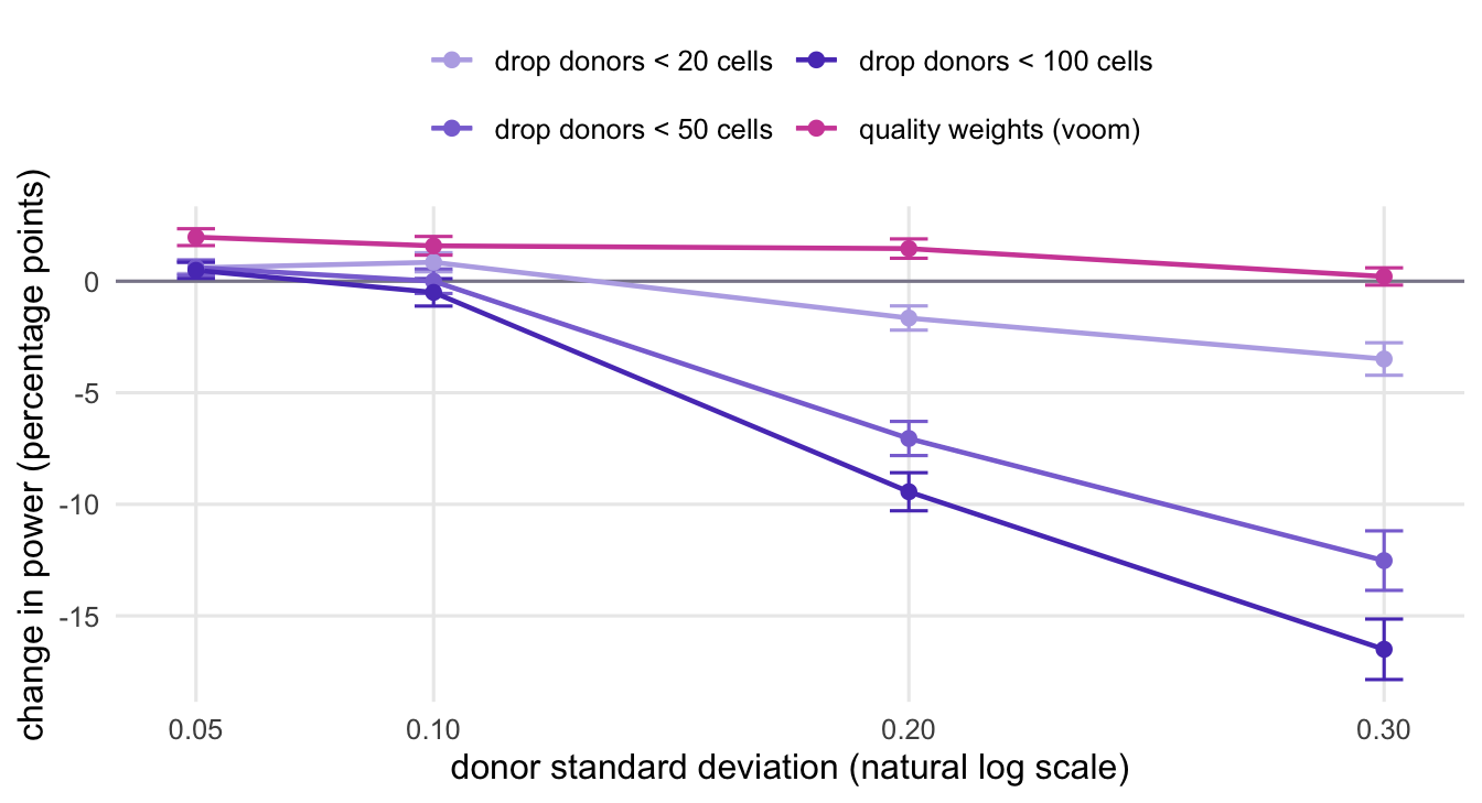
In the main simulation, then, the 12-cell donor adds little noise beyond what the count model already expects from its smaller library, and removing small donors removes replicates. Dropping donors below 20 cells lowered edgeR’s power by 3.6 percentage points, below 50 cells by 12.6 and below 100 by 16.3. The quality weights agree: voomWithQualityWeights() gave the 12-cell donor an average weight of 0.84 and the 800-cell donor 0.96, and changed power by 0.6 percentage points relative to plain voom.
Figure 4 repeats the comparison with 40 experiments at each of 4 sizes of donor variation. When donors are very alike, the small pseudobulks become the noisiest samples, and both remedies help a little: at a donor standard deviation of 0.05, dropping donors below 50 cells raised power by 0.6 percentage points and the quality weights by 2.0, while the quality weights gave the 12-cell donor an average weight of 0.56 (the 800-cell donor 1.30). As donor variation grows, the floors turn into a loss, and a large one, while the quality weights stay at or slightly above zero. Down-weighting is the safer of the two because it is estimated from the data, and it gives a noisy pseudobulk less say instead of deleting a replicate.
Figure 4: Change in power from dropping small donors (edgeR QL, compared with keeping every donor) and from sample quality weights (voomWithQualityWeights, compared with plain voom), as donor-to-donor variation grows. Bars show two Monte Carlo standard errors of the paired difference.
What to do in practice
Sum the raw counts per donor within each cell type and give the sums, unchanged, to edgeR, DESeq2 or limma-voom. In Seurat that is AggregateExpression(); on a plain count matrix, rowsum() on the transposed matrix does it, as in aggregate_donors() above. Do not divide by the number of cells, do not round averages, and do not give AverageExpression() output to a count model: the library size already accounts for the number of cells, and it does so without losing the count scale.
Keep the number of cells behind each pseudobulk next to the counts, and look at it before choosing a floor. A fixed floor in a small design mostly removes replicates. Whether a small pseudobulk is a problem depends on how much donors differ, and the data can tell you: with a quality-weights fit, a small pseudobulk that is truly noisier gets a visibly lower weight, and the down-weighted analysis keeps its information instead of discarding it.
# pb: genes x donors matrix of summed raw counts for one cell type# (AggregateExpression(...)$RNA, or t(rowsum(t(counts), donor)))# condition: factor with one entry per column of pb; n_cells: cells behind each columndesign <-model.matrix(~ condition)y <-DGEList(pb, group = condition)keep <-filterByExpr(y, design)y <-normLibSizes(y[keep, , keep.lib.sizes =FALSE])fit <-glmQLFit(y, design, robust =TRUE, legacy =FALSE)res <-glmQLFTest(fit, coef =2)topTags(res)# are the small pseudobulks the noisy ones?vq <-voomWithQualityWeights(y, design)data.frame(n_cells, weight =round(vq$targets$sample.weights, 2))# if they are, the weighted limma fit is a reasonable main analysisfit_w <-eBayes(lmFit(vq, design))topTable(fit_w, coef =2)
If a pseudobulk analysis finds too few genes, the remedy is more donors; more cells per donor help only while the cell-level and counting noise are still large next to the donor-to-donor variation.
The simulation script
All the functions shown above live in pseudobulk_sim.R. Running that file as a script (Rscript pseudobulk_sim.R) repeats the experiments and writes pseudobulk_sim-results.csv, which the table and the figures read; the scoring function and the loop are below.
Scoring: FPR, observed FDR, power and fold-change error
score_methods <-function(out, sim, alpha =0.05) { keep <-attr(out, "keep"); de <- sim$is_de; truth <- sim$lfc2 lfc_set <- de & keep # true DE genes that were testedt(vapply(out, function(o) { padj <-if (!is.null(o$padj)) o$padj elsep.adjust(o$p, "BH") call <-!is.na(padj) & padj < alpha fd <-sum(call &!de); td <-sum(call & de) ok <- lfc_set &is.finite(o$lfc) # a method may give no estimatec(fpr =mean(o$p[!de & keep] < alpha, na.rm =TRUE),calls = fd + td, fdp = fd /max(fd + td, 1), power = td /sum(de),rmse =sqrt(mean((o$lfc[ok] - truth[ok])^2)),slope =unname(coef(lm(o$lfc[ok] ~0+ truth[ok]))),lfc_missing =1-sum(ok) /sum(lfc_set)) }, numeric(7)))}
The Monte Carlo loop (run as a script; it writes the results file)
if (sys.nframe() ==0L) { alpha <-0.05 n_main <-as.integer(Sys.getenv("PB_NMAIN", "60")) # data sets, main setting n_sweep <-as.integer(Sys.getenv("PB_NSWEEP", "40")) # data sets per sweep setting sweep_sd <-c(0.05, 0.1, 0.2, 0.3)# does the DESeq2 default dispersion fit cope with rounded means? (log only) default_fit <-function(sim, agg) { keep <-filterByExpr(DGEList(agg$sums, group = sim$group), model.matrix(~ sim$group)) cnt <-round(agg$means[keep, ]); storage.mode(cnt) <-"integer" dds <-DESeqDataSetFromMatrix(cnt, data.frame(g = sim$group), ~ g) msg <-character(0) res <-tryCatch(withCallingHandlers( {DESeq(dds, quiet =TRUE); "ok"},message =function(m) {msg <<-c(msg, conditionMessage(m)); invokeRestart("muffleMessage")},warning =function(w) invokeRestart("muffleWarning")),error =function(e) "error")if (res =="ok"&&any(grepl("local regression fit was automatically substituted", msg))) res <-"fallback" res } main <-vector("list", n_main); weights <-matrix(NA_real_, n_main, 8) zero_share <-numeric(n_main); genewise <-logical(n_main); default_status <-character(n_main)for (i inseq_len(n_main)) {set.seed(1000+ i) sim <-sim_cells() agg <-aggregate_donors(sim) out <-run_methods(sim, agg) main[[i]] <-score_methods(out, sim) weights[i, ] <- out$sum_voomqw$weights zero_share[i] <- out$mean_deseq2$zero_share genewise[i] <- out$mean_deseq2$route =="gene-wise" default_status[i] <-default_fit(sim, agg)cat("main", i, "\n") }# power differences within each data set: floors vs no floor, quality weights vs voom paired <-function(a) { d <-rbind(floor20 = a["floor20", "power", ] - a["sum_edger", "power", ],floor50 = a["floor50", "power", ] - a["sum_edger", "power", ],floor100 = a["floor100", "power", ] - a["sum_edger", "power", ],voomqw = a["sum_voomqw", "power", ] - a["sum_voom", "power", ])c(setNames(rowMeans(d), paste0(rownames(d), "_mean")),setNames(apply(d, 1, sd) /sqrt(ncol(d)), paste0(rownames(d), "_se"))) } arr <-simplify2array(main) # method x metric x data set mc_mean <-apply(arr, 1:2, mean) mc_se <-apply(arr, 1:2, sd) /sqrt(n_main) sweep_rows <-list()for (sd_i in sweep_sd) { sc <-lapply(seq_len(n_sweep), function(i) {set.seed(round(5000+1000* sd_i *100) + i) sim <-sim_cells(donor_sd = sd_i) out <-run_methods(sim, aggregate_donors(sim), deseq =FALSE, mean_log =FALSE)list(score =score_methods(out, sim), weights = out$sum_voomqw$weights) }) a <-simplify2array(lapply(sc, `[[`, "score")) w <-colMeans(do.call(rbind, lapply(sc, `[[`, "weights"))) sweep_rows[[as.character(sd_i)]] <-list(mean =apply(a, 1:2, mean),se =apply(a, 1:2, sd) /sqrt(n_sweep),diff =paired(a),weights =setNames(w, paste0("weight_donor", 1:8)))cat("sweep", sd_i, "\n") } flat <-function(m, prefix) { v <-as.vector(m)setNames(v, paste(prefix, rep(rownames(m), ncol(m)), rep(colnames(m), each =nrow(m)),sep ="_")) } vals <-c(flat(mc_mean, "main"), flat(mc_se, "mainse"),setNames(paired(arr), paste0("maindiff_", names(paired(arr)))),setNames(colMeans(weights), paste0("qw_weight_donor", 1:8)),zero_share_mean =mean(zero_share),default_ok =sum(default_status =="ok"),default_fallback =sum(default_status =="fallback"),default_error =sum(default_status =="error"),genewise_route =sum(genewise),n_main = n_main, n_sweep = n_sweep)for (k innames(sweep_rows)) { vals <-c(vals, flat(sweep_rows[[k]]$mean, paste0("sweep", k)),flat(sweep_rows[[k]]$se, paste0("sweepse", k)),setNames(sweep_rows[[k]]$diff, paste0("sweepdiff", k, "_", names(sweep_rows[[k]]$diff))),setNames(sweep_rows[[k]]$weights, paste0("sweep", k, "_", names(sweep_rows[[k]]$weights)))) } res <-data.frame(name =names(vals), value =sprintf("%.10g", vals)) ver <-data.frame(name =c("R_version", "edgeR_version", "limma_version", "DESeq2_version"),value =c(paste(R.version$major, R.version$minor, sep ="."),as.character(packageVersion("edgeR")),as.character(packageVersion("limma")),as.character(packageVersion("DESeq2")))) out_file <-Sys.getenv("PB_OUT", "pseudobulk_sim-results.csv")write.csv(rbind(res, ver), out_file, row.names =FALSE, quote =FALSE)}