qPCR statistics for the delta delta Ct method: run the t-test on delta Ct values, not on 2^-ddCt fold changes, and never count technical wells as replicates.
You ran a qPCR experiment, computed for every animal, and now you want a p-value. Do you run the t-test on the fold changes, or on the delta Ct values? And what about the common habit of setting every control to 1?
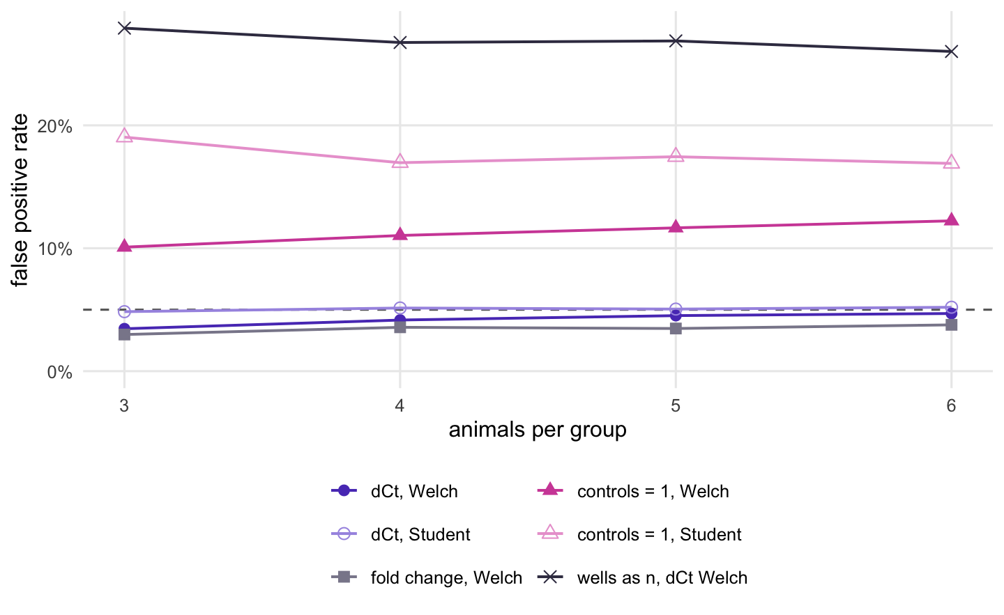
Run the test on the delta Ct values, and convert only the final estimate and its confidence interval into a fold change. In the simulation below, with three animals per group and no true effect, a t-test on delta Ct gives a false positive in 4.8% of experiments (Student) or 3.5% (Welch): at or below 5%, as it should. A t-test on the fold changes also stays below 5%, but it misses real effects more often: with six animals per group it detects a true two-fold increase in 55.1% of experiments, against 65.5% on delta Ct. Setting the controls to exactly 1 and testing the treated fold changes against them gives 10.1%, or 19.0% with Student’s t-test. Counting the 3 technical wells of each animal as separate replicates gives 27.9%.
Ct, delta Ct and delta delta Ct
A qPCR machine records, for each well, the cycle at which the fluorescence crosses a threshold: the Ct (cycle threshold; newer software calls it Cq, the quantification cycle). More starting template means an earlier crossing, so a lower Ct means more transcript, and if the reaction doubles its product every cycle, one cycle less means twice as much.
The delta Ct of a sample is the Ct of the target gene minus the Ct of a reference gene measured in the same sample, . It removes whatever affects both genes equally, such as how much RNA went into the reverse transcription. The delta delta Ct is the difference between the group means of delta Ct, treated minus control, and is the fold change (Livak & Schmittgen 2001). A delta delta Ct of is a two-fold increase.
The formula assumes a doubling every cycle, that is 100% amplification efficiency. If your primer efficiencies are measured and differ from that, each gene’s Ct difference becomes the exponent of that gene’s own efficiency instead of 2 (Pfaffl 2001). The log of that ratio is still a linear combination of Ct values, so the statistics still belong on the log scale.
The simulation
Each simulated experiment has control and treated animals, a target gene and a reference gene, and 3 wells per gene per animal. The Ct values are built from four sources of variation:
n_wells <-3# technical replicate wells per gene per samplect_target <-26# typical Ct of the target genect_ref <-20# typical Ct of the reference genesd_input <-0.5# sample-to-sample differences in RNA input and cDNA yield (both genes)sd_target <-0.6# biological variation of the target between animalssd_ref <-0.2# biological variation of the reference genesd_well <-0.2# pipetting and well-to-well noisetrue_ddct <--1# treated target Ct one cycle lower: a two-fold increasen_example <-4# animals per group in the worked example
All variation is normal on the Ct scale (log-normal on the linear scale), the usual working model for qPCR. The input term is shared by both genes, so delta Ct removes it. The reference gene does not respond to the treatment, and both groups have the same spread. Those last two assumptions matter: a reference gene that moves with treatment biases every method here equally, and unequal spread is the case where Welch’s version of the t-test earns its keep.
In fold terms, one standard deviation between animals moves the target by a factor of 1.52, and one standard deviation of well noise by 1.15. Treat this as one plausible setting, not a benchmark: outbred animals and human samples usually vary more, and a second run further down raises the between-animal spread to stand for that case.
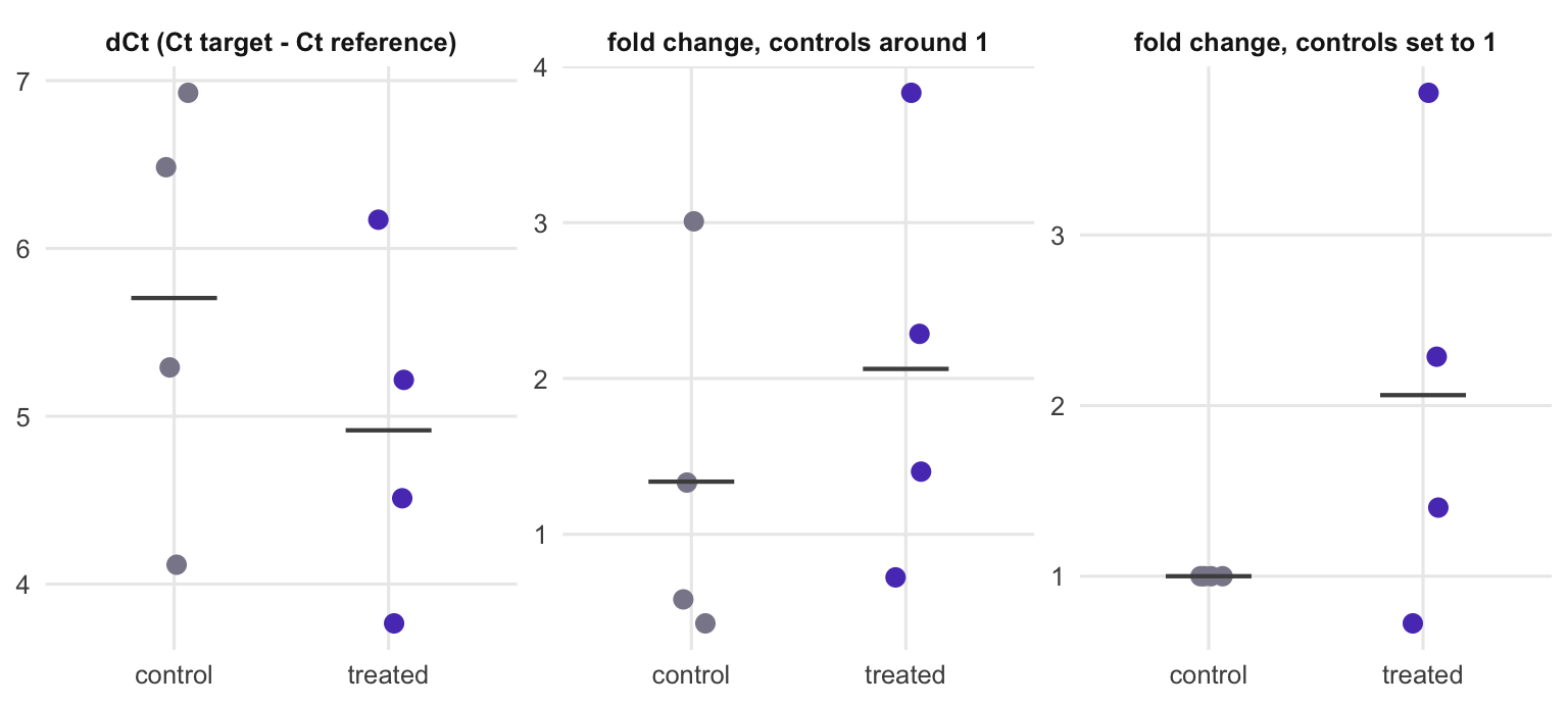
Here is one experiment with 4 animals per group and a true two-fold increase. Wells are averaged on the Ct scale, then each animal gets a delta Ct and a fold change relative to the mean control delta Ct.
simulate_plate <-function(n, ddct) { group <-factor(rep(c("control", "treated"), each = n), levels =c("control", "treated")) input <-rnorm(2* n, 0, sd_input) # shared by both genes of a sample mu_t <- ct_target + input +rnorm(2* n, 0, sd_target) + ddct * (group =="treated") mu_r <- ct_ref + input +rnorm(2* n, 0, sd_ref) wells <-expand.grid(well =seq_len(n_wells), sample =seq_len(2* n))data.frame(sample = wells$sample, well = wells$well, group = group[wells$sample],ct_target = mu_t[wells$sample] +rnorm(nrow(wells), 0, sd_well),ct_ref = mu_r[wells$sample] +rnorm(nrow(wells), 0, sd_well))}set.seed(20260930)plate <-simulate_plate(n = n_example, ddct = true_ddct)head(plate, 4)
  sample well   group ct_target   ct_ref
1      1    1 control  27.19099 20.78575
2      1    2 control  27.17695 20.81989
3      1    3 control  27.32331 20.63357
4      2    1 control  24.90869 19.82468
# average the technical wells on the Ct scale, then dCt = Ct target - Ct referenceper_sample <-aggregate(cbind(ct_target, ct_ref) ~ sample + group, data = plate, FUN = mean)per_sample$dct <- per_sample$ct_target - per_sample$ct_refctrl <- per_sample$group =="control"trt <- per_sample$group =="treated"per_sample$ddct <- per_sample$dct -mean(per_sample$dct[ctrl])per_sample$fc <-2^-per_sample$ddctper_sample[, c("sample", "group", "dct", "ddct", "fc")]
  sample   group      dct       ddct        fc
1      1 control 6.484015  0.7796075 0.5825253
2      2 control 5.290907 -0.4135000 1.3319132
3      3 control 4.115430 -1.5889774 3.0083604
4      4 control 6.927277  1.2228699 0.4284296
5      5 treated 6.171159  0.4667522 0.7235917
6      6 treated 4.511414 -1.1929930 2.2862656
7      7 treated 5.216803 -0.4876042 1.4021145
8      8 treated 3.765943 -1.9384640 3.8329734
ex_ctrl_mean <-mean(per_sample$fc[ctrl])
The controls scatter around 1, but their average is 1.34. They were centred on the delta Ct scale, so their geometric mean is exactly 1, and the arithmetic mean of such values is always larger: a cycle below the mean adds more on the linear scale than a cycle above takes away.
One experiment, three tests
Three analyses a reader might run on this table: a t-test on delta Ct, a t-test on the per-animal fold changes, and the “controls = 1” version, with every control entered as exactly 1.
# (1) the log-scale test: Welch t-test on dCttt_dct <-t.test(per_sample$dct[trt], per_sample$dct[ctrl])# (2) t-test on the per-sample fold changes 2^-ddCttt_fc <-t.test(per_sample$fc[trt], per_sample$fc[ctrl])# (3) every control set to exactly 1, then a t-test against the treated fold changestt_one <-t.test(per_sample$fc[trt], rep(1, sum(ctrl)))c(dct = tt_dct$p.value, fold_change = tt_fc$p.value, controls_at_1 = tt_one$p.value)
The three p-values are 0.37, 0.45 and 0.21. From the delta Ct test the estimated fold change is 1.73, with a 95% confidence interval from 0.43 to 6.97. With this much variation a true two-fold change can easily go undetected in one experiment. The figure shows what each analysis sees.
ex <-rbind(data.frame(panel ="dCt (Ct target - Ct reference)", group = per_sample$group,value = per_sample$dct),data.frame(panel ="fold change, controls around 1", group = per_sample$group,value = per_sample$fc),data.frame(panel ="fold change, controls set to 1", group = per_sample$group,value =ifelse(ctrl, 1, per_sample$fc)))ex$panel <-factor(ex$panel, levels =unique(ex$panel))ggplot(ex, aes(group, value, colour = group)) +geom_point(size =2.8, position =position_jitter(width =0.08, height =0, seed =1)) +stat_summary(fun = mean, geom ="crossbar", width =0.4, linewidth =0.3, colour ="grey30") +facet_wrap(~panel, scales ="free_y") +scale_colour_manual(values =c(control ="#8a889a", treated ="#5a3fc0"), guide ="none") +labs(x =NULL, y =NULL) + theme_pc
Figure 1: One simulated experiment shown three ways. Left: delta Ct per animal, where lower means more target. Middle: the same animals as fold changes relative to the control mean delta Ct. Right: the controls entered as exactly 1. Bars mark group means.
Two facts, checked in the next chunk, explain most of what follows.
# dividing every value by the same constant does not change a t-testlin <-2^-per_sample$dctp_raw <-t.test(lin[trt], lin[ctrl])$p.valuep_norm <-t.test(per_sample$fc[trt], per_sample$fc[ctrl])$p.value# a Welch test against a constant group is the one-sample test against 1one_welch <-t.test(per_sample$fc[trt], rep(1, sum(ctrl)))one_samp <-t.test(per_sample$fc[trt], mu =1)one_stud <-t.test(per_sample$fc[trt], rep(1, sum(ctrl)), var.equal =TRUE)stopifnot(isTRUE(all.equal(p_raw, p_norm)),isTRUE(all.equal(one_welch$p.value, one_samp$p.value)),isTRUE(all.equal(unname(one_stud$statistic), unname(one_samp$statistic))))c(df_one_sample =unname(one_samp$parameter), df_student =unname(one_stud$parameter))
First, normalising to the control mean multiplies every by the same constant, which a t-test ignores: test (2) is simply a t-test on linear expression values.
Second, entering the controls as a column of 1s turns the comparison into something else. R’s t.test() uses Welch’s test unless you pass var.equal = TRUE (checked in the chunk). A group with no variance adds nothing to Welch’s standard error, and the result is identical to a one-sample t-test of the treated fold changes against 1. Student’s version gives the same t statistic but, because it pools the zero variance of the controls, it credits the test with 6 degrees of freedom instead of 3. Either way the uncertainty in the control mean has disappeared, and with equal group sizes that is half of the variance of the difference between the two means.
Ten thousand experiments without an effect
The next chunks simulate 10,000 experiments for each group size from 3 to 6 animals per group, with no effect and with a true two-fold increase. The tests are vectorised for speed and checked against t.test(). Three variants join the three analyses above: Student’s t-test on delta Ct, Student’s t-test with the controls entered as 1, and a Welch test that treats each well as a replicate (each target well paired with a reference well of the same animal, so 3 delta Ct values per animal).
# the same simulation for many experiments at once: rows = experimentsrow_var <-function(X) rowSums((X -rowMeans(X))^2) / (ncol(X) -1)two_sample <-function(X, Y, equal_var =FALSE) { # Welch or Student, as t.test() nx <-ncol(X); ny <-ncol(Y); vx <-row_var(X); vy <-row_var(Y) est <-rowMeans(X) -rowMeans(Y)if (equal_var) { se <-sqrt(((nx -1) * vx + (ny -1) * vy) / (nx + ny -2) * (1/ nx +1/ ny)) df <-rep(nx + ny -2, nrow(X)) } else { se <-sqrt(vx / nx + vy / ny) df <- se^4/ ((vx / nx)^2/ (nx -1) + (vy / ny)^2/ (ny -1)) } q <-qt(0.975, df)data.frame(p =2*pt(-abs(est / se), df), lo = est - q * se, hi = est + q * se, est = est)}one_sample <-function(X, mu) { n <-ncol(X); m <-rowMeans(X); se <-sqrt(row_var(X) / n); q <-qt(0.975, n -1)data.frame(p =2*pt(-abs((m - mu) / se), n -1), lo = m - q * se, hi = m + q * se,est = m - mu, se = se)}simulate_many <-function(n_sim, n, ddct, sd_t = sd_target, sd_w = sd_well) { N <-2* n; treated <-rep(c(FALSE, TRUE), each = n) input <-matrix(rnorm(n_sim * N, 0, sd_input), n_sim) mu_t <- ct_target + input +matrix(rnorm(n_sim * N, 0, sd_t), n_sim) + ddct *rep(treated, each = n_sim) mu_r <- ct_ref + input +matrix(rnorm(n_sim * N, 0, sd_ref), n_sim) well_noise <-function() rnorm(n_sim * N * n_wells, 0, sd_w)list(ct_t =array(mu_t, c(n_sim, N, n_wells)) +well_noise(), # experiment x sample x wellct_r =array(mu_r, c(n_sim, N, n_wells)) +well_noise(),treated = treated)}analyse_many <-function(s, ddct) { ic <-!s$treated; it <- s$treated; fc_true <-2^-ddct dct <-rowMeans(s$ct_t, dims =2) -rowMeans(s$ct_r, dims =2) # wells averaged on Ct scale fc <-2^-(dct -rowMeans(dct[, ic])) # per-sample 2^-ddCt well_dct <-matrix(s$ct_t - s$ct_r, nrow(dct)) # one dCt per well pair well_t <-rep(it, n_wells) res <-list("dCt, Welch"=two_sample(dct[, it], dct[, ic]),"dCt, Student"=two_sample(dct[, it], dct[, ic], equal_var =TRUE),"fold change, Welch"=two_sample(fc[, it], fc[, ic]),"controls = 1, Welch"=one_sample(fc[, it], 1),"controls = 1, Student"=two_sample(fc[, it], matrix(1, nrow(fc), sum(ic)), equal_var =TRUE),"wells as n, dCt Welch"=two_sample(well_dct[, well_t], well_dct[, !well_t]),# the same "controls = 1" test on the log scale: treated ddCt against 0, no skew"controls = 1, log scale"=one_sample(dct[, it] -rowMeans(dct[, ic]), 0))# does the reported 95% interval contain the true fold change?# dCt intervals are on the ddCt scale; "fold change, Welch" reports the ratio of means,# 1 + (difference of means) / (control mean); "controls = 1" reports the treated mean cm <-rowMeans(fc[, ic]) covers <-c("dCt, Welch"=mean(res[[1]]$lo <= ddct & res[[1]]$hi >= ddct),"dCt, Student"=mean(res[[2]]$lo <= ddct & res[[2]]$hi >= ddct),"fold change, Welch"=mean(1+ res[[3]]$lo / cm <= fc_true &1+ res[[3]]$hi / cm >= fc_true),"controls = 1, Welch"=mean(res[[4]]$lo <= fc_true & res[[4]]$hi >= fc_true),"controls = 1, Student"=NA_real_,"wells as n, dCt Welch"=mean(res[[6]]$lo <= ddct & res[[6]]$hi >= ddct),"controls = 1, log scale"=mean(res[[7]]$lo <= ddct & res[[7]]$hi >= ddct))# the error bar most figures show: treated mean fold change +/- one SEM sem_cover <-mean(res[[4]]$est +1- res[[4]]$se <= fc_true & res[[4]]$est +1+ res[[4]]$se >= fc_true)data.frame(method =names(res), reject =sapply(res, function(r) mean(r$p <0.05)),reject_up =sapply(res, function(r) mean(r$p <0.05& r$est >0)),coverage = covers, sem_cover = sem_cover, row.names =NULL)}
# the vectorised tests give the same p-values as t.test() on the first experimentsset.seed(1)chk <-simulate_many(20, n =4, ddct =0)dct_chk <-rowMeans(chk$ct_t, dims =2) -rowMeans(chk$ct_r, dims =2)p_vec <-two_sample(dct_chk[, chk$treated], dct_chk[, !chk$treated])$pp_ref <-sapply(1:20, function(i) t.test(dct_chk[i, chk$treated], dct_chk[i, !chk$treated])$p.value)p_vec1 <-one_sample(dct_chk[, chk$treated], 0)$pp_ref1 <-sapply(1:20, function(i) t.test(dct_chk[i, chk$treated])$p.value)stopifnot(isTRUE(all.equal(p_vec, p_ref)), isTRUE(all.equal(p_vec1, p_ref1)))
n_sim <-10000n_values <-3:6set.seed(20260930)runs <-do.call(rbind, lapply(n_values, function(n) rbind(cbind(n = n, scenario ="null", analyse_many(simulate_many(n_sim, n, 0), 0)),cbind(n = n, scenario ="two-fold", analyse_many(simulate_many(n_sim, n, true_ddct), true_ddct)))))# a noisier biology: target biological SD of 1 cycle, six animals per groupsd_noisy <-1noisy <-analyse_many(simulate_many(n_sim, 6, true_ddct, sd_t = sd_noisy), true_ddct)# wells as n with tighter and noisier wells, three animals per group, no effectsd_w_tight <-0.1; sd_w_loose <-0.5wells_tight <-analyse_many(simulate_many(n_sim, 3, 0, sd_w = sd_w_tight), 0)wells_loose <-analyse_many(simulate_many(n_sim, 3, 0, sd_w = sd_w_loose), 0)# "controls = 1" with large groups, no effectn_big <-20big <-analyse_many(simulate_many(n_sim, n_big, 0), 0)mc_se <-sqrt(0.05*0.95/ n_sim) # Monte Carlo standard error of a 5% rateruns$method <-factor(runs$method, levels =c(names(method_cols), "controls = 1, log scale"))
Figure 2: False positive rate with no true effect, by group size and analysis. The dashed line is the nominal level of the test.
With 10,000 experiments per point, a rate of 5% is measured with a standard error of 0.22%, so differences of a percentage point or more are real.
Both delta Ct tests hold their level. Student’s stays between 4.8% and 5.2% at every group size, 5% within the precision of the simulation, and Welch’s is a little conservative with small groups (3.5% with three animals, 4.7% with six). The t-test on fold changes runs between 3.0% and 3.8%: no inflation, and its cost shows up in the next section.
Setting the controls to 1 does inflate them, from 10.1% with three animals per group to 12.2% with six in the Welch (equivalently, one-sample) form. The main cause is the one shown above: the control mean is treated as known, so with equal group sizes the standard error is too small by a factor of the square root of 2. The chunk below checks this by running the same test on the log scale, the treated delta delta Ct values against 0, where nothing is skewed. Its rate matches the exact rate for a standard error that is too small by that factor (9.3% against 9.3% with three animals, 12.7% against 12.9% with six). The climb with group size comes from the t distribution: more degrees of freedom lower the critical value, so the same wrong standard error rejects more often, heading towards 16.6% for very large groups.
The skew of the fold changes is a second, smaller effect, and at these group sizes it does not push the test towards “up”: more null experiments are rejected downwards than upwards (7.1% against 3.0% with three animals, 6.8% against 5.4% with six). The upward bias of the skewed mean only takes over with large groups: with 20 animals per group, the fold change version rejects 18.9% of null experiments, 15.6% of them upwards, against 16.3% on the log scale. Student’s form is worse at every group size tested (19.0% with three animals, 16.9% with six), because of the extra degrees of freedom it credits.
# "controls = 1": the same test on the log scale, the exact rate if the only fault is a# standard error too small by sqrt(2), and the direction of the linear-scale rejectionsctl <-data.frame(n =c(n_values, n_big))ctl$log_scale <-c(sapply(n_values, rate, m ="controls = 1, log scale"), big_log)ctl$sqrt2_rule <-th(ctl$n)ctl$fold_scale <-c(sapply(n_values, rate, m ="controls = 1, Welch"), big_lin)ctl$fold_up <-c(sapply(n_values, rate, m ="controls = 1, Welch", what ="reject_up"), big_up)ctl$fold_down <- ctl$fold_scale - ctl$fold_upctl[-1] <-lapply(ctl[-1], pc)ctl
Counting wells as replicates is the worst of all, between 26.0% and 27.9% at every group size tested. Wells measure one animal several times; they do not measure several animals. In this simulation 83% of the variance of a single well-pair delta Ct lies between animals, not between wells, so tripling n shrinks the standard error without shrinking the real uncertainty. How bad it gets depends on that share. With tighter wells (standard deviation 0.1 cycles, 95% of the variance between animals) the rate with three animals rises to 32.5%; with noisier wells (0.5 cycles, 44%) it falls to 16.0%, still far above 5%. This is the same mistake as treating cells as replicates in single-cell data (see pseudobulk versus cell-level tests).
Power, and the interval you report
The same simulation with a true two-fold increase measures power, and how often the reported 95% interval contains the true fold change.
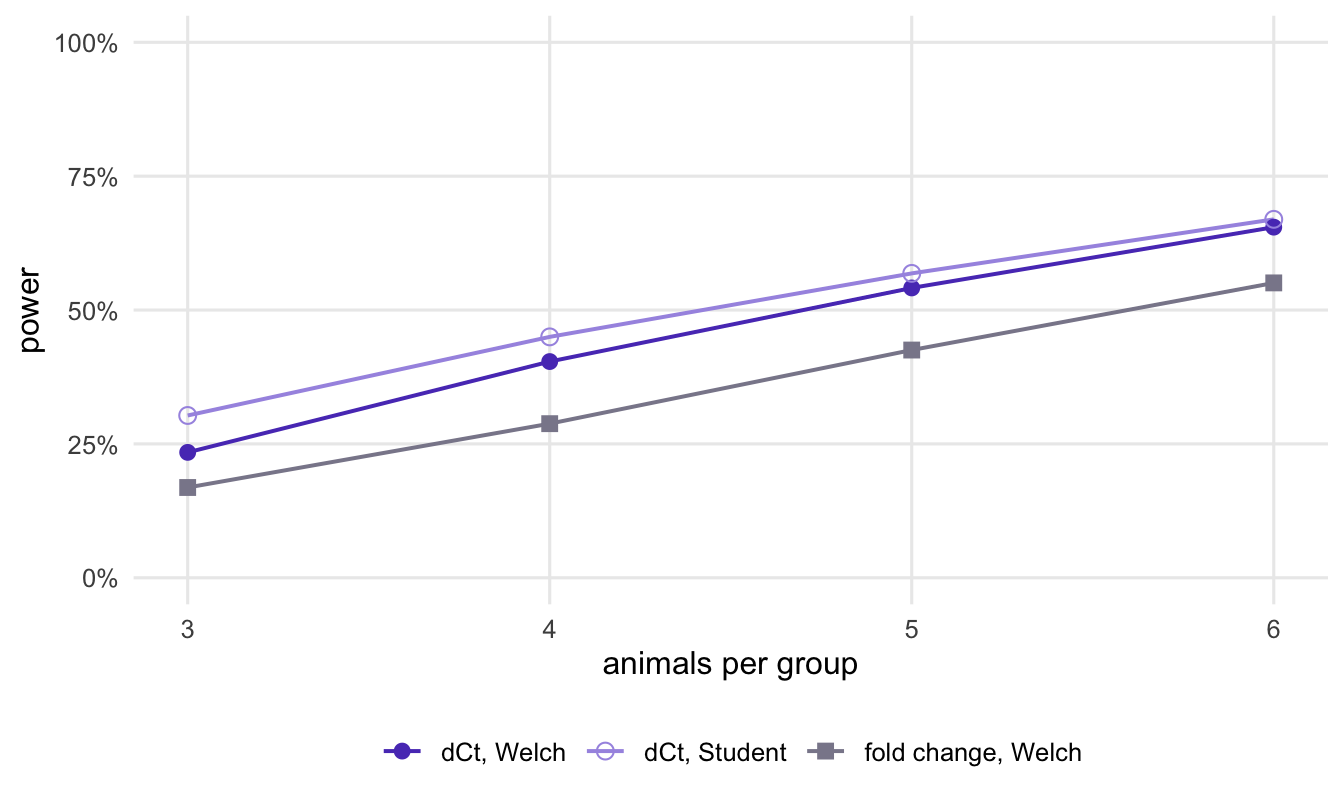
Figure 3: Power to detect a true two-fold increase at the 5% level, for the three analyses that hold their false positive rate.
Testing on delta Ct finds the effect more often. With six animals per group, Welch’s test on delta Ct detects the two-fold change in 65.5% of experiments and the t-test on fold changes in 55.1%; with three animals the figures are 23.4% and 16.9%. Student’s test on delta Ct has more power than Welch’s with three animals (30.3% against 23.4%), the price of not assuming equal variances; by six the gap is small (66.9% against 65.5%). The inflated tests are left out on purpose: “controls = 1” with six animals reaches 69.1%, but it also rejects 12.2% of true nulls.
ggplot(subset(runs, scenario =="two-fold"&!is.na(coverage) & method %in%names(method_cols)),aes(n, coverage, colour = method, shape = method)) +geom_hline(yintercept =0.95, linetype ="dashed", colour ="grey40") +geom_line(linewidth =0.7) +geom_point(size =2.6) +scale_colour_manual(values = method_cols, name =NULL) +scale_shape_manual(values = method_shapes, name =NULL) +scale_y_continuous(labels =function(x) paste0(100* x, "%")) +guides(colour =guide_legend(ncol =2)) +labs(x ="animals per group", y ="coverage of the 95% interval") + theme_pc
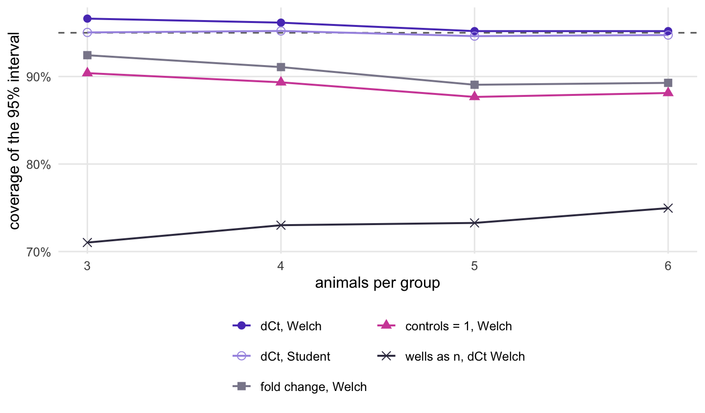
Figure 4: How often the reported 95% confidence interval for the fold change contains the true fold change, with a true two-fold increase. Delta Ct intervals are back-transformed; the fold change interval is the simple linear-scale one described in the text.
The interval from the delta Ct test, back-transformed with at both ends, covers the true fold change in 96.6% of experiments with three animals and 95.2% with six (Student: 95.0% and 94.7%). It is not symmetric around the fold change, and should not be: “half as much” and “twice as much” are not the same distance from 1.
The fold change interval here is the simple one a spreadsheet gives: the Welch interval for the difference between the group means of the fold changes, divided by the control mean as if that mean were known. The “controls = 1” interval is the mean of the treated fold changes plus or minus its t-based margin. Both fall short, and further short with six animals than with three: 92.4% and 89.3% for the first, 90.4% and 88.1% for the second. Better-built ratio intervals exist, but they take more than a spreadsheet formula, and the back-transformed delta Ct interval already has the right coverage. The wells-as-replicates interval, 71.0% to 75.0%, is far too narrow for the same reason its test is too eager.
Most published bar charts show neither interval. They show the mean fold change plus or minus one standard error (SEM). Drawn around the treated mean in the “controls = 1” style, that bar contains the true fold change in 43.9% of experiments with three animals per group and 47.0% with six.
The size of these differences depends on how variable your animals are. In a second run with the target’s biological standard deviation raised from 0.6 to 1 cycle and six animals per group, the delta Ct test detects the two-fold change in 32.1% of experiments and the fold change test in 20.4%, and the fold change interval covers the truth in 89.7% of experiments against 95.8% for delta Ct. The more skewed the fold changes, the more the linear scale costs.
What to do in practice
Average technical wells on the Ct scale, one value per gene per biological sample. Compute delta Ct per sample. Run the test on delta Ct, and report the fold change and its interval by back-transforming:
# per_sample: one row per animal, with its group and its delta Ct (wells already averaged)fit <-t.test(dct ~ group, data = per_sample) # Welch; var.equal = TRUE for Studentddct_hat <-unname(fit$estimate[2] - fit$estimate[1]) # treated minus controlc(fold_change =2^-ddct_hat,lower =2^-(-fit$conf.int[1]), # conf.int is for control - treatedupper =2^-(-fit$conf.int[2]))
With the formula interface, t.test() estimates the first factor level minus the second, here control minus treated, hence the negation. Check the sign against your group means.
Plot the delta Ct values, or plot fold changes on a log axis, so the picture matches the test. If you want the controls shown at 1, draw them as fold changes relative to their own mean, as in the middle panel of the first figure, with their spread visible. With independent animals, never enter them into the test as a column of 1s.
Cell culture is often different. If each experiment (a run, a passage, a plate) has its own control and its own treated sample, and each treated sample is normalised to its own control, the controls are 1 by design and the data are paired. The right test is then the paired t-test on delta Ct, which is the same as a one-sample t-test of the per-experiment delta delta Ct values against 0, on the Ct scale, not on the fold changes:
# pretend the example's animals came as four experiments, each with one control and one treatedrun_ddct <- per_sample$dct[trt] - per_sample$dct[ctrl]p_paired <-t.test(per_sample$dct[trt], per_sample$dct[ctrl], paired =TRUE)$p.valuep_onesam <-t.test(run_ddct, mu =0)$p.valuestopifnot(isTRUE(all.equal(p_paired, p_onesam)))
An unpaired test would throw away the pairing and lose power when experiments differ a lot.
Yuan and colleagues describe the same analysis (delta Ct per sample, then a two-group t-test) alongside regression and ANCOVA models that estimate delta delta Ct directly (Yuan et al. 2006). The regression form extends to more than two groups: fit lm(dct ~ group) and back-transform the coefficients and their confint() intervals with . With a large panel of targets (a few dozen or more) measured on the same samples, limma can fit that model to every target at once, and its eBayes() step moderates each gene’s standard error towards a common value. With a handful of targets that common value is poorly estimated, and targets normalised to the same reference gene share its noise.