Seurat DE: integrated, SCT or RNA assay?

scRNA-seq
Seurat
integration
pseudobulk
edgeR
Which Seurat assay should differential expression use after integration or SCTransform? A simulation shows the integrated assay shrinks condition effects.
Author

Pseudocount

Published

3 November 2026

Setup: packages and helper functions
suppressPackageStartupMessages(library(ggplot2))
stopifnot(packageVersion("ggplot2") >= "3.4.0")
violet <- "#5a3fc0"; magenta <- "#d14fa6"; grey <- "#8a8799"
fmt_num <- function(x, d = 2) sprintf(paste0("%.", d, "f"), x)
fmt_pct <- function(x, d = 0) sprintf(paste0("%.", d, "f%%"), 100 * x)
fmt_int <- function(x) format(round(x), big.mark = ",", trim = TRUE)
theme_set(theme_minimal(base_size = 12) +
  theme(panel.grid.minor = element_blank(),
        plot.background = element_rect(fill = "white", colour = "white"),
        strip.text = element_text(face = "bold")))
Read the simulation results
res <- read.csv("integration_sim-results.csv", stringsAsFactors = FALSE)
v <- setNames(res$value, res$name)
num <- function(k) as.numeric(v[[k]])
n_seeds <- num("n_seeds"); seeds <- seq_len(n_seeds)
per_seed <- function(k) sapply(seeds, function(s) num(paste0(k, "_seed", s)))
layers <- c(rna = "RNA assay", integrated = "integrated assay", sct = "SCT assay",
            pseudobulk = "pseudobulk (edgeR)")
slopes <- sapply(names(layers), function(l) per_seed(paste0("slope_", l)))
methods <- c(cell_rna = "RNA", cell_integrated = "integrated", cell_sct = "SCT",
             mean_rna = "RNA", mean_integrated = "integrated", mean_sct = "SCT",
             pseudobulk = "summed counts")
tp <- sapply(names(methods), function(m) per_seed(paste0("tp_", m)))
fp <- sapply(names(methods), function(m) per_seed(paste0("fp_", m)))
ari_raw <- per_seed("ari_unintegrated"); ari_int <- per_seed("ari_integrated")
n_genes <- num("n_genes"); n_de <- num("n_de"); n_null <- n_genes - n_de
cells_per_sample <- num("cells_per_sample"); batch_sd <- num("batch_sd")
n_per_group <- num("n_per_group"); n_samples <- 2 * n_per_group
type_prob <- c(A = num("type_prob_A"), B = num("type_prob_B"), C = num("type_prob_C"))
marker_fold <- num("marker_fold"); lfc_min <- num("lfc_min"); lfc_max <- num("lfc_max")
alpha <- num("alpha")
n_cells_A <- per_seed("n_cells_A")
n_int_genes <- per_seed("n_int_genes"); n_sct_genes <- per_seed("n_sct_genes")
v5_assays <- v[["v5_assays"]]; v5_reductions <- v[["v5_reductions"]]
seurat_v <- v[["seurat_version"]]; edger_v <- v[["edger_version"]]
limma_v <- v[["limma_version"]]; sctransform_v <- v[["sctransform_version"]]
genes <- read.csv("integration_sim-genes.csv")
Summaries quoted in the text
slope_mean <- colMeans(slopes)
slope_rng <- apply(slopes, 2, range)
tp_mean <- colMeans(tp); fp_mean <- colMeans(fp)
g_de <- genes[genes$is_de, ]                  # genes with a true effect, data set 1

You have integrated your samples in Seurat and annotated the clusters, and now you want the genes that change between treated and control cells inside one cluster. The object has more than one assay: RNA, and perhaps SCT or one called integrated. Which one should FindMarkers() or any other differential expression (DE) test use?

Not the integrated one. In the simulation below, each sample comes from one condition, as in most real studies. Measured on the integrated assay, the true condition effects shrank to 22% of their size on average (between 18% and 27% across 6 simulated data sets). The RNA assay and a pseudobulk analysis of the raw counts kept them close to full size. Integration is for the embedding and the clusters; the differential expression goes back to the counts. Seurat’s own vignettes give the same advice: the v4 integration vignette switches back to the original data for differential expression after integration, and the current one recommends aggregating cells from the same sample and subpopulation (pseudobulking) for comparisons across conditions. This post measures what happens if you do not.

Which workflow makes which object

The answer depends on which Seurat workflow produced your object, so it helps to know what each one creates.

In the Seurat v5 workflow (Hao et al. 2024) the RNA assay is split into one layer per sample, and IntegrateLayers() with method = CCAIntegration (or RPCAIntegration, HarmonyIntegration, JointPCAIntegration) returns a corrected low-dimensional reduction, nothing else. In the simulation, the object after IntegrateLayers() has the assay “RNA” and the reductions “pca integrated.cca”: there is no corrected expression matrix to test. This was checked in the source of Seurat 5.0.1 and 5.5.1, where each of these integration methods returns only the new reduction, and the integration vignette says the same. With these four methods, a v5 user never meets the question “integrated or RNA” unless they chose the older route. FastMNNIntegration from the SeuratWrappers package is different: it also writes a reconstructed expression assay (mnn.reconstructed by default), which holds corrected values, and the caution below applies to it as well.

That older route, FindIntegrationAnchors() followed by IntegrateData(), still exists in Seurat 5 and is what many tutorials and saved objects use. It creates a new assay called integrated whose data layer holds corrected log-normalised values (after the SCT route, normalization.method = "SCT", it holds corrected Pearson residuals in scale.data instead, according to its help page). Two details matter here. By default the assay contains only the anchor features, the variable genes chosen for finding anchors, so in real data many genes are not in it at all. (The simulated data sets below have few enough genes that all 1,500 made it in.) And the correction is built from pairs of cells matched across samples, the anchors: for each pair, the difference between their expression profiles is computed, weighted, and subtracted from the cells being integrated (Stuart et al. 2019).

SCTransform (Hafemeister and Satija 2019) is a normalisation, not an integration, but it is often run as part of one. In Seurat v5 with split layers it fits one model per sample (the source loops over the layers). Its data layer holds the log of corrected counts and scale.data holds Pearson residuals. FindMarkers() on the SCT assay uses the data layer by default, and it stops with an error when the per-sample models were fitted at different sequencing depths until you run PrepSCTFindMarkers(), which recomputes the corrected counts at one common depth.

The setup

# Integrated, SCT or RNA assay for differential expression: the simulation behind the post.
# Run from the post folder: Rscript integration_sim.R
# Writes integration_sim-results.csv (name,value) and integration_sim-genes.csv (per gene, seed 1).
# Runtime: several minutes per seed (SCTransform without glmGamPoi and the anchor integration
# are the slow steps).
# Expect many warnings. Without the glmGamPoi package, SCTransform falls back to its native fit,
# which warns "iteration limit reached" and "alternation limit reached"; installing glmGamPoi
# removes most of them. IntegrateData() warns "Different cells in new layer data than already
# exists for scale.data" (suppressed below). Both are harmless here.
suppressPackageStartupMessages({
  library(Seurat)
  library(edgeR)
  library(limma)
  library(Matrix)
})
stopifnot(packageVersion("Seurat") >= "5.0.0", packageVersion("SeuratObject") >= "5.0.0",
          packageVersion("edgeR") >= "4.0.0", packageVersion("limma") >= "3.58.0",
          packageVersion("mclust") >= "6.0.0")
options(Seurat.presto.wilcox.msg = FALSE, future.globals.maxSize = 2e9)
alpha <- 0.05
seeds <- 1:6

# ---- simulated counts -----------------------------------------------------------------------
# 2 control and 2 treated samples, 3 cell types, negative binomial counts. Every gene gets a
# random shift per sample (the sample effect), the same in all cell types. The first n_de genes
# change with treatment, in cell type A only, by a known log2 fold change.
simulate <- function(seed, n_genes = 1500, cells_per_sample = 500, n_per_group = 2,
                     type_prob = c(A = 0.5, B = 0.3, C = 0.2), n_marker = 80, marker_fold = 4,
                     n_de = 100, lfc_range = c(0.5, 2), batch_sd = 0.3, phi = 0.2) {
  set.seed(seed)
  n_samples <- 2 * n_per_group
  samples <- sprintf("s%d", seq_len(n_samples))
  cond_s <- rep(c("ctrl", "trt"), each = n_per_group)
  types <- names(type_prob)
  sample <- rep(samples, each = cells_per_sample)
  celltype <- sample(types, length(sample), replace = TRUE, prob = type_prob)
  mu0 <- exp(rnorm(n_genes, log(0.3), 1.2))                  # baseline mean UMI per cell
  type_eff <- matrix(0, n_genes, length(types))             # marker genes of each type
  for (k in seq_along(types))
    type_eff[n_de + (k - 1) * n_marker + seq_len(n_marker), k] <- log(marker_fold)
  lfc2 <- c(sample(c(-1, 1), n_de, TRUE) * runif(n_de, lfc_range[1], lfc_range[2]),
            rep(0, n_genes - n_de))
  batch <- matrix(rnorm(n_genes * n_samples, 0, batch_sd), n_genes, n_samples)
  depth <- exp(rnorm(length(sample), 0, 0.3)) *
    rep(exp(rnorm(n_samples, 0, 0.3)), each = cells_per_sample)  # cell and sample depth
  si <- match(sample, samples)
  trt_A <- as.numeric(cond_s[si] == "trt" & celltype == "A")
  eta <- log(mu0) + type_eff[, match(celltype, types)] + batch[, si] +
    outer(lfc2 * log(2), trt_A)
  m <- exp(eta) * rep(depth, each = n_genes)
  counts <- matrix(rnbinom(length(m), mu = m, size = 1 / phi), n_genes)
  dimnames(counts) <- list(sprintf("g%04d", seq_len(n_genes)),
                           sprintf("c%05d", seq_along(sample)))
  meta <- data.frame(sample = sample, condition = cond_s[si], celltype = celltype,
                     row.names = colnames(counts))
  list(counts = counts, meta = meta, lfc2 = setNames(lfc2, rownames(counts)),
       is_de = setNames(seq_len(n_genes) <= n_de, rownames(counts)))
}

# ---- helpers --------------------------------------------------------------------------------
# cell-level FindMarkers, treated vs control cells of type A, every gene tested
find_markers_A <- function(obj, assay, genes) {
  Idents(obj) <- paste(obj$celltype, obj$condition, sep = "_")
  fm <- FindMarkers(obj, ident.1 = "A_trt", ident.2 = "A_ctrl", assay = assay,
                    slot = "data", logfc.threshold = 0, min.pct = 0, verbose = FALSE)
  fm[genes, ]                               # genes absent from the assay give empty rows
}
# per-sample means of a layer in type A, then limma-trend (samples as replicates)
sample_means_limma <- function(x, meta, genes) {
  x <- x[intersect(genes, rownames(x)), ]
  a <- meta$celltype == "A"
  mm <- sapply(split(which(a), meta$sample[a]), function(j) rowMeans(x[, j, drop = FALSE]))
  g <- factor(meta$condition[match(colnames(mm), meta$sample)])
  fit <- eBayes(lmFit(mm, model.matrix(~ g)), trend = TRUE)
  tt <- topTable(fit, coef = 2, number = nrow(mm), sort.by = "none")
  setNames(tt$adj.P.Val, rownames(tt))[genes]  # genes absent from the layer: not called
}
# pseudobulk: summed raw counts per sample in type A, edgeR quasi-likelihood
pseudobulk_edger <- function(counts, meta) {
  a <- meta$celltype == "A"
  pb <- t(rowsum(t(counts[, a]), meta$sample[a]))
  g <- factor(meta$condition[match(colnames(pb), meta$sample)])
  design <- model.matrix(~ g)
  y <- DGEList(pb, group = g)
  keep <- filterByExpr(y, design)
  y <- normLibSizes(y[keep, , keep.lib.sizes = FALSE])
  fit <- glmQLFit(y, design, robust = TRUE, legacy = FALSE)
  tab <- glmQLFTest(fit, coef = 2)$table
  lfc <- fdr <- setNames(rep(NA_real_, nrow(pb)), rownames(pb))
  lfc[rownames(tab)] <- tab$logFC
  fdr[rownames(tab)] <- p.adjust(tab$PValue, "BH")
  list(lfc = lfc, fdr = fdr)
}
slope_through_origin <- function(est, truth) unname(coef(lm(est ~ 0 + truth)))

# ---- one simulated data set -----------------------------------------------------------------
run_one <- function(seed) {
  sim <- simulate(seed)
  de <- names(which(sim$is_de)); null <- names(which(!sim$is_de))
  so <- CreateSeuratObject(as(sim$counts, "CsparseMatrix"), meta.data = sim$meta)

  # Seurat v5 workflow: layers split by sample, IntegrateLayers() for the embedding
  v5 <- so
  v5[["RNA"]] <- split(v5[["RNA"]], f = v5$sample)
  v5 <- NormalizeData(v5, verbose = FALSE)
  v5 <- FindVariableFeatures(v5, verbose = FALSE)
  v5 <- ScaleData(v5, verbose = FALSE)
  v5 <- RunPCA(v5, npcs = 20, verbose = FALSE)
  v5 <- IntegrateLayers(v5, method = CCAIntegration, orig.reduction = "pca",
                        new.reduction = "integrated.cca", verbose = FALSE)
  v5_assays <- paste(Assays(v5), collapse = " ")
  v5_reductions <- paste(Reductions(v5), collapse = " ")
  ari <- sapply(c(unintegrated = "pca", integrated = "integrated.cca"), function(r) {
    x <- FindNeighbors(v5, reduction = r, dims = 1:20, verbose = FALSE)
    x <- FindClusters(x, resolution = 0.1, verbose = FALSE)
    mclust::adjustedRandIndex(x$seurat_clusters, x$celltype)
  })
  v5 <- JoinLayers(v5)                                # one "data" layer again, for DE
  fm_rna <- find_markers_A(v5, "RNA", rownames(so))

  # Seurat v4-style workflow: anchors + IntegrateData() creates the "integrated" assay
  ol <- lapply(SplitObject(so, split.by = "sample"), function(x)
    FindVariableFeatures(NormalizeData(x, verbose = FALSE), verbose = FALSE))
  feats <- SelectIntegrationFeatures(ol, verbose = FALSE)
  anchors <- FindIntegrationAnchors(ol, anchor.features = feats, verbose = FALSE)
  int <- suppressWarnings(IntegrateData(anchors, verbose = FALSE))
  int <- int[, colnames(so)]
  n_int_genes <- nrow(int[["integrated"]])
  fm_int <- find_markers_A(int, "integrated", rownames(so))

  # SCTransform, one model per sample, then PrepSCTFindMarkers() before FindMarkers()
  sct <- so
  sct[["RNA"]] <- split(sct[["RNA"]], f = sct$sample)
  sct <- suppressMessages(SCTransform(sct, verbose = FALSE))
  sct <- PrepSCTFindMarkers(sct, verbose = FALSE)
  fm_sct <- find_markers_A(sct, "SCT", rownames(so))
  n_sct_genes <- nrow(sct[["SCT"]])

  # the same layers, averaged per sample, with the sample as the replicate
  genes <- rownames(so)
  lm_rna <- sample_means_limma(LayerData(v5, assay = "RNA", layer = "data"), sim$meta, genes)
  lm_int <- sample_means_limma(LayerData(int, assay = "integrated", layer = "data"),
                               sim$meta, genes)
  lm_sct <- sample_means_limma(LayerData(sct, assay = "SCT", layer = "data"), sim$meta, genes)
  pb <- pseudobulk_edger(sim$counts, sim$meta)

  lfc <- list(rna = fm_rna$avg_log2FC, integrated = fm_int$avg_log2FC,
              sct = fm_sct$avg_log2FC, pseudobulk = pb$lfc)
  lfc <- lapply(lfc, setNames, rownames(so))
  q <- list(cell_rna = p.adjust(fm_rna$p_val, "BH"), cell_integrated = p.adjust(fm_int$p_val, "BH"),
            cell_sct = p.adjust(fm_sct$p_val, "BH"), mean_rna = lm_rna, mean_integrated = lm_int,
            mean_sct = lm_sct, pseudobulk = pb$fdr)
  q <- lapply(q, function(v) setNames(v, rownames(so))[rownames(so)])
  called <- lapply(q, function(v) !is.na(v) & v < alpha)
  out <- c(
    setNames(sapply(lfc, function(e) slope_through_origin(e[de], sim$lfc2[de])),
             paste0("slope_", names(lfc))),
    setNames(sapply(called, function(k) sum(k[de])), paste0("tp_", names(called))),
    setNames(sapply(called, function(k) sum(k[null])), paste0("fp_", names(called))),
    ari_unintegrated = ari[["unintegrated"]], ari_integrated = ari[["integrated"]],
    n_int_genes = n_int_genes, n_sct_genes = n_sct_genes, n_cells_A = sum(sim$meta$celltype == "A"))
  genes <- data.frame(gene = rownames(so), is_de = sim$is_de, true_lfc = sim$lfc2,
                      lfc_rna = lfc$rna, lfc_integrated = lfc$integrated,
                      lfc_sct = lfc$sct, lfc_pseudobulk = lfc$pseudobulk)
  message("seed ", seed, " done")
  list(out = out, genes = genes, v5_assays = v5_assays, v5_reductions = v5_reductions)
}

res <- lapply(seeds, run_one)
num <- do.call(rbind, lapply(seq_along(seeds), function(i)
  data.frame(name = paste0(names(res[[i]]$out), "_seed", seeds[i]), value = unname(res[[i]]$out))))
f <- lapply(formals(simulate)[-1], eval)
meta_rows <- data.frame(
  name = c("n_seeds", "n_genes", "n_de", "cells_per_sample", "batch_sd", "alpha",
           "n_per_group", paste0("type_prob_", names(f$type_prob)), "n_marker", "marker_fold",
           "lfc_min", "lfc_max",
           "v5_assays", "v5_reductions", "r_version", "seurat_version", "seuratobject_version",
           "sctransform_version", "edger_version", "limma_version", "glmgampoi_installed"),
  value = c(length(seeds), f$n_genes, f$n_de, f$cells_per_sample, f$batch_sd, alpha,
            f$n_per_group, f$type_prob, f$n_marker, f$marker_fold, f$lfc_range,
            res[[1]]$v5_assays, res[[1]]$v5_reductions,
            paste(R.version$major, R.version$minor, sep = "."),
            as.character(packageVersion("Seurat")), as.character(packageVersion("SeuratObject")),
            as.character(packageVersion("sctransform")), as.character(packageVersion("edgeR")),
            as.character(packageVersion("limma")),
            as.character(requireNamespace("glmGamPoi", quietly = TRUE))))
write.csv(rbind(meta_rows, num), "integration_sim-results.csv", row.names = FALSE)
write.csv(res[[1]]$genes, "integration_sim-genes.csv", row.names = FALSE)
The script above simulates the data and runs every analysis in this post. It is not run when the page is built (it takes several minutes per data set); the page reads the numbers it saved. They were computed with Seurat 5.0.1, sctransform 0.4.1, edgeR 4.0.16 and limma 3.58.1.

Each simulated data set has 4 samples, 2 control and 2 treated, with 500 cells each and 1,500 genes. Counts are negative binomial, the usual model for UMI counts. There are three cell types, A, B and C, making up on average 50%, 30% and 20% of the cells, each with its own marker genes expressed 4 times higher than in the other types.

Two things differ between samples. The first is a sample effect: every gene in every sample is shifted up or down at random, by a standard deviation of 0.3 on the natural log scale, and the shift is the same in all three cell types. This stands for everything that makes one sample differ from another apart from the treatment: library preparation, time to dissociation, the donor’s genotype. The second is the treatment: the first 100 genes change in treated samples, in cell type A only, by a log2 fold change drawn uniformly between 0.5 and 2, up or down. The other 1,400 genes have no treatment effect.

The assumption that drives everything below is that each sample is entirely one condition. The integration unit (the sample) and the condition line up, so nothing in the data can tell the treatment apart from the sample effect except the design, which integration does not see.

Each data set went through three standard workflows: the v5 route (split layers, IntegrateLayers() with CCA, clustering, then JoinLayers() so that DE can run on the RNA assay), the v4-style route (IntegrateData(), giving the integrated assay), and SCTransform per sample followed by PrepSCTFindMarkers(). The comparison is always treated against control cells of type A.

Integration did what it is for. Clusters built on the unintegrated PCA agreed poorly with the true cell types: the adjusted Rand index (1 means perfect agreement) was 0.29 on average. On the integrated CCA reduction it was 0.998 or higher in every data set. So the question is not whether to integrate, but what to use the result for.

The common way: DE on the integrated assay

long <- do.call(rbind, lapply(names(layers), function(l)
  data.frame(layer = layers[[l]], truth = g_de$true_lfc, est = g_de[[paste0("lfc_", l)]])))
long$layer <- factor(long$layer, levels = layers)
fit_lines <- data.frame(layer = factor(layers, levels = layers), slope = slopes[1, ])
ggplot(long, aes(truth, est)) +
  geom_point(colour = violet, alpha = 0.45, size = 1.6, na.rm = TRUE) +
  geom_abline(slope = 1, intercept = 0, linetype = "dashed", colour = "grey30") +
  geom_abline(data = fit_lines, aes(slope = slope, intercept = 0), colour = violet,
              linewidth = 1) +
  facet_wrap(~ layer, nrow = 2) +
  labs(x = "true log2 fold change", y = "estimated log2 fold change")
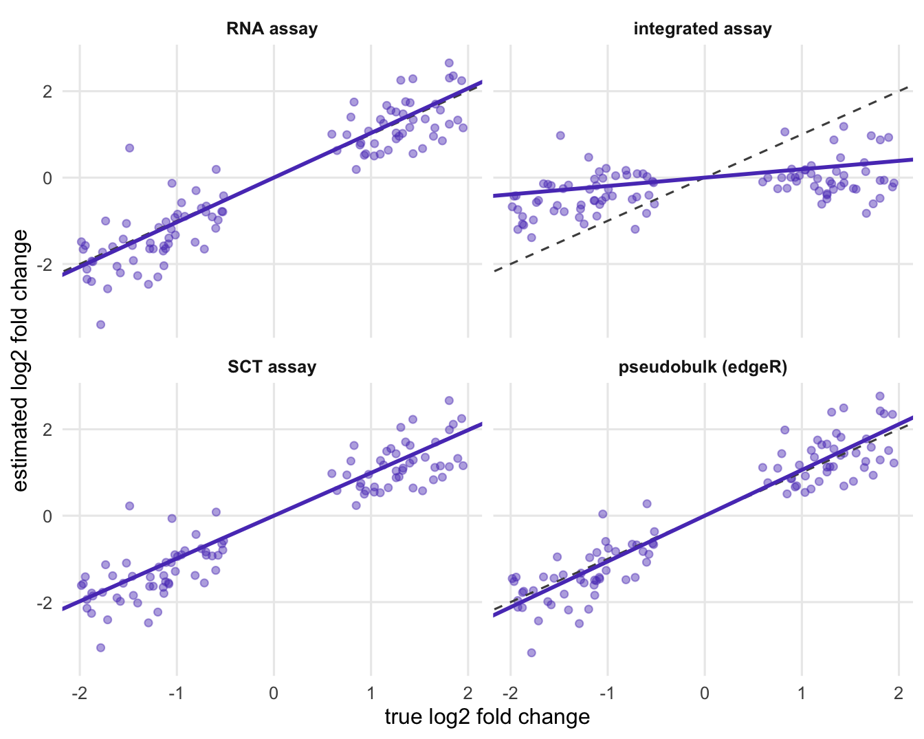
Four scatter panels of estimated versus true log2 fold change. In the RNA assay, SCT assay and pseudobulk panels the points follow the dashed diagonal; in the integrated assay panel they lie on a much flatter line close to zero.
Figure 1: Estimated against true log2 fold change for the genes with a true treatment effect, in the first simulated data set. The dashed line is perfect recovery; the violet line is the fitted slope through the origin. Genes removed by filterByExpr are not shown in the pseudobulk panel.
Slopes per simulated data set
tab <- data.frame(data_set = seeds, round(slopes, 2))
names(tab) <- c("data set", layers)
knitr::kable(tab)
data set RNA assay integrated assay SCT assay pseudobulk (edgeR)
1 1.03 0.19 0.99 1.06
2 1.05 0.22 1.21 1.05
3 0.98 0.18 0.95 0.96
4 0.97 0.19 0.95 0.96
5 0.89 0.25 0.86 0.91
6 1.02 0.27 0.98 1.03

Figure 1 shows the first data set. The y axis is the avg_log2FC column that FindMarkers() reports for treated against control cells of type A (for the pseudobulk panel, the edgeR log fold change). On the RNA assay the genes follow the diagonal, with a fitted slope of 1.03. On the integrated assay the same genes lie on a line with slope 0.19. At that slope, a true 4-fold change (a log2 fold change of 2) is reported as about 1.3-fold.

The table repeats the measurement on all 6 data sets. The integrated assay kept between 18% and 27% of the true effect. The RNA assay ranged from 0.89 to 1.05, pseudobulk from 0.91 to 1.06, and the SCT assay from 0.86 to 1.21.

The reason is the way the correction works. A treated cell of type A finds its anchors among control cells of type A in the other samples, because those are the cells that look most like it. The difference between the two is the sample effect plus the treatment effect, and IntegrateData() subtracts it. Nothing in the method can tell that part of the difference is the biology you want: when a treatment affects every cell of a sample, to the anchors it looks exactly like a batch effect. Removing sample differences is the job integration is asked to do, and here the treatment is a sample difference. The direction of the result follows from this mechanism; the size of the shrinkage depends on the setup (how large the sample effect is, how many genes are anchor features, how many cell types the treatment touches), so the percentage above belongs to this simulation, not to every data set.

One more detail makes this easy to fall into: IntegrateData() sets the new assay as the default (checked in the source of both Seurat versions above), so a FindMarkers() call without an assay argument runs on the integrated values unless you switch back to RNA.

Which genes get called

shown <- c("cell_rna", "cell_integrated", "cell_sct", "pseudobulk")
grp <- ifelse(grepl("^cell_", shown), "cells as replicates (FindMarkers)",
              "samples as replicates")
lab <- ifelse(grepl("^cell_", shown), paste(methods[shown], "assay"), "summed counts (edgeR)")
dd <- data.frame(label = rep(lab, 2), group = rep(grp, 2),
                 kind = rep(c("true treatment gene", "no true effect"), each = length(lab)),
                 n = c(tp_mean[shown], fp_mean[shown]))
dd$label <- factor(dd$label, levels = rev(lab))
dd$kind <- factor(dd$kind, levels = c("no true effect", "true treatment gene"))
dd$group <- factor(dd$group, levels = unique(grp))
ggplot(dd, aes(n, label, fill = kind)) +
  geom_col(width = 0.65) +
  facet_wrap(~ group, ncol = 1, scales = "free") +
  scale_fill_manual(values = c("true treatment gene" = violet, "no true effect" = magenta),
                    breaks = c("true treatment gene", "no true effect")) +
  labs(x = "genes called per data set (mean)", y = NULL, fill = NULL) +
  theme(legend.position = "top", strip.text = element_text(hjust = 0))
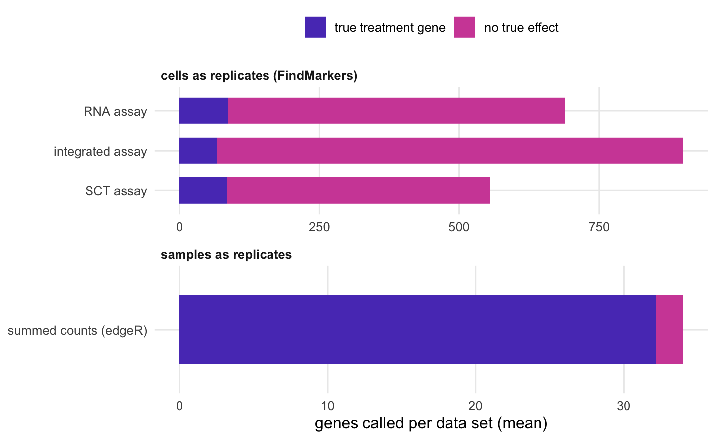
Horizontal stacked bars. In the top group, cell-level tests on the RNA, SCT and integrated assays each call hundreds of genes, most of them magenta false calls, with the integrated assay calling the most false genes. In the bottom panel, on a much shorter axis, the single bar for summed counts with edgeR is almost entirely violet true calls with a thin magenta end.
Figure 2: Genes called at the Benjamini-Hochberg FDR threshold used in the text, averaged over the simulated data sets, split into genes with a true treatment effect and genes without one. Top: cells as replicates (FindMarkers on each assay). Bottom: summed counts per sample with edgeR, on its own, much shorter axis.

Effect sizes are half of the picture; the list of significant genes is what people act on. Figure 2 counts the genes called at a Benjamini-Hochberg FDR of 5%, averaged over the 6 data sets.

FindMarkers() treats each cell as a replicate. With about 503 treated and as many control cells of type A per data set, the sample effect alone looks significant, so every assay calls hundreds of genes that have no treatment effect (this is the subject of the post on cell-level tests). Integration does not rescue this. On the integrated assay the cell-level test called 833 null genes per data set on average, against 603 on the RNA assay, and found fewer of the true ones (67 of 100, against 86). Removing the sample effect from the values does not turn cells into independent replicates.

Making the sample the replicate changes the picture. Summing the raw counts of type A cells per sample and running edgeR’s quasi-likelihood pipeline (Chen et al. 2016) found 32.2 of the 100 true genes per data set on average, with 1.8 false calls. With 2 samples per condition that is a modest yield, and an honest one: the true effects have to be seen against the sample-to-sample variation, and so few replicates do not pin that variation down well. A benchmark on real data found that methods which aggregate cells within each replicate before testing performed best (Squair et al. 2021).

The script also averages each layer per sample and tests the 4 means with limma-trend. With 2 samples per condition those calls were too unstable to compare layers: on the RNA assay they ranged from 0 to 25 true genes, with none at all in 3 of the 6 data sets, so they are not shown. The effect sizes above are the cleaner measure of what integration did.

What the SCT assay does

The SCT assay behaved like the RNA assay. After PrepSCTFindMarkers(), its avg_log2FC values kept the true effects (slopes between 0.86 and 1.21). SCTransform fitted one model per sample, but the model is about sequencing depth, and here the corrected counts kept the treatment difference between samples. Its problem is the same as the RNA assay’s: FindMarkers() on SCT still treats cells as replicates.

Two limits of this check. The scale.data layer (Pearson residuals) was not measured, because FindMarkers() does not use it by default. And the container that ran the script did not have the glmGamPoi package, so SCTransform used its slower built-in fitting (glmgampoi_installed in the results file); a machine with glmGamPoi can give slightly different SCT numbers. The other Seurat numbers can also move a little between Seurat versions.

When integration is harmless

Integration is not the problem. The integrated reduction (in v5) or the integrated assay (in the older route) is the right input for everything that is about which cells are alike: the neighbour graph, the clusters, the UMAP, label transfer. Those need the sample effect removed, and in this simulation clustering needed integration to recover the cell types.

The problem starts when the corrected values are used as expression measurements to compare conditions that line up with the integration unit. That is the usual design, because a mouse or a patient is either treated or not. Designs in which every sample contains cells of both conditions were not simulated here, and the argument above does not carry over to them unchanged.

What to do in practice

Integrate for the embedding and the clusters, then go back to the counts for differential expression. In a Seurat v5 object with sample and condition columns in the metadata:

library(Seurat)
library(edgeR)
obj[["RNA"]] <- split(obj[["RNA"]], f = obj$sample)
obj <- NormalizeData(obj)
obj <- FindVariableFeatures(obj)
obj <- ScaleData(obj)
obj <- RunPCA(obj)
obj <- IntegrateLayers(obj, method = CCAIntegration, orig.reduction = "pca",
                       new.reduction = "integrated.cca")
obj <- FindNeighbors(obj, reduction = "integrated.cca", dims = 1:30)
obj <- FindClusters(obj)
obj <- JoinLayers(obj)          # one counts layer again, for DE and for plots

# one cluster: sum the raw counts per sample, then edgeR quasi-likelihood
cells <- WhichCells(obj, idents = "0")
counts <- LayerData(obj, assay = "RNA", layer = "counts")[, cells]
sample_of_cell <- factor(obj$sample[cells])
pb <- as.matrix(Matrix::tcrossprod(counts, Matrix::fac2sparse(sample_of_cell)))
condition <- factor(obj$condition[match(colnames(pb), obj$sample)])
design <- model.matrix(~ condition)
y <- DGEList(pb, group = condition)
keep <- filterByExpr(y, design)
y <- normLibSizes(y[keep, , keep.lib.sizes = FALSE])
fit <- glmQLFit(y, design, robust = TRUE, legacy = FALSE)
res <- glmQLFTest(fit, coef = 2)
topTags(res)

The tcrossprod() line adds up each sample’s counts without making the whole count matrix dense. Seurat’s own AggregateExpression(obj, assays = "RNA", group.by = c("sample", "seurat_clusters")), which the current vignette uses, gives the same sums for all clusters at once (on the test object below, its result for one cluster matched the tcrossprod() sums exactly); check its column names, which combine the sample and cluster labels. legacy = FALSE selects the quasi-likelihood method introduced in edgeR 4.0; it is the default in current edgeR but not in the 4.0 series, so it is written out. This block was run on a small simulated object before being put here.

If your object came from IntegrateData(), set DefaultAssay(obj) <- "RNA" before any DE call or expression plot, and do the pseudobulk step on the RNA counts as above. For violin plots, dot plots and feature plots, the log-normalised data layer of the RNA assay is the natural choice; the integrated values are corrected towards the other samples and do not show what was measured.

If the pseudobulk analysis finds fewer genes than the cell-level test did, that is the size of the answer your samples support. More samples per condition is what raises it.

References

Stuart T, Butler A, Hoffman P et al. 2019 Cell 177(7):1888-1902.e21 (doi:10.1016/j.cell.2019.05.031)

Hao Y, Stuart T, Kowalski MH et al. 2024 Nature Biotechnology 42(2):293-304 (doi:10.1038/s41587-023-01767-y)

Hafemeister C, Satija R 2019 Genome Biology 20(1):296 (doi:10.1186/s13059-019-1874-1)

Squair JW, Gautier M, Kathe C et al. 2021 Nature Communications 12(1):5692 (doi:10.1038/s41467-021-25960-2)

Chen Y, Lun ATL, Smyth GK 2016 F1000Research 5:1438 (doi:10.12688/f1000research.8987.2)

The numbers on this page were computed with the versions below.

R version 4.5.3 (2026-03-11)
Bioconductor 3.22
ggplot2 4.0.3