Which background (universe) should GO enrichment use in clusterProfiler or limma? Simulated data show the whole genome invents terms; use the genes you tested.
Author
Pseudocount
Published
17 November 2026
Setup: packages and helper functions
suppressPackageStartupMessages({library(limma)library(edgeR)library(DESeq2)library(ggplot2)})stopifnot(packageVersion("limma") >="3.50", packageVersion("edgeR") >="4.0.0",packageVersion("DESeq2") >="1.36", packageVersion("ggplot2") >="3.4.0")pct <-function(x, d =0) sprintf(paste0("%.", d, "f%%"), 100* x)num <-function(x) format(round(x), big.mark =",", scientific =FALSE, trim =TRUE)dec <-function(x, d =2) sprintf(paste0("%.", d, "f"), x)theme_pc <-function() theme_minimal(base_size =12) +theme(panel.grid.minor =element_blank(), strip.text =element_text(face ="bold"),plot.background =element_rect(fill ="white", colour ="white"))uni_lab <-c(genome ="whole genome", annotated ="annotated genes", tested ="tested genes")uni_col <-c(genome ="#d14fa6", annotated ="#8e8c9c", tested ="#5a3fc0")# the limma default this post mentions, read from the installed packagekegga_restrict <-eval(formals(getS3method("kegga", "default"))$restrict.universe)
You have a list of differentially expressed (DE) genes and you want to know which Gene Ontology (GO) terms are over-represented in it. The test needs a background, often called the universe: the set of genes the DE list is compared against. Which genes should it contain? The genes that could have ended up in the DE list, which means the genes your DE analysis actually tested. In the simulation below no gene set is truly enriched. With the whole genome as the background, the test still called 4.1 gene sets per experiment on average, and at least one in 87.5% of the experiments. With the tested genes as the background, at least one set was called in 1.5% of the experiments, within the 5% the correction promises.
This is not an obscure point. When Wijesooriya and colleagues (2022) screened published articles, nearly all of the analyses that used over-representation tests either had no appropriate background list or did not say which one they used.
What the test compares
Over-representation analysis asks, for each gene set (a GO term, a pathway), whether it holds more DE genes than you would expect if the DE list were a random draw from the universe. For one set the data form a two-by-two table: genes in the set or not, DE or not. The p-value is the chance of seeing at least the observed overlap under that random draw, which is a one-sided hypergeometric test, the same as a one-sided Fisher’s exact test.
The random-draw model is where the background comes in. An RNA-seq experiment on liver cannot call a gene DE if the gene is not expressed in liver: it has no reads, or too few, and is filtered out before the test. The DE list is drawn from expressed genes only. If the background is the whole genome, a set whose members are mostly expressed in the tissue will hold more DE genes than the test expects, with no biology behind it. If a share of a set’s members is expressed and a share of the background is, the set receives on average times the overlap that the test expects. With 60% of the genome expressed, as below, a set of genes that are all expressed receives 1.67 times the expected overlap. That excess is real and reproducible, so with enough DE genes the test finds it.
The setup
Each simulated experiment starts from a fresh annotation of 20,000 genes, of which 60% are expressed in the tissue. I assume that exactly these genes pass the expression filter and are tested for differential expression; real filters do not line up with biology this neatly, which is the subject of a later section. Genes can carry annotation with a chance of 90% if they are expressed and 50% if not, a crude version of the fact that well-studied genes tend to be broadly expressed. From these genes I build 400 GO-like gene sets of 15 to 400 members. Each set has its own tissue share, the share of its members that are expressed: its expected value is drawn between 20% and 100%, and the realised share varies around it. Members are drawn independently for each set, so sets overlap, as GO terms do.
In the main scenario the DE list is a random draw of 1,200 genes from the tested genes, 10% of them. Among the genes that were tested, then, no set is enriched. In a second scenario one set of 100 genes is truly enriched: its tested members are 3 times as likely to be DE as other tested genes. Its tissue share is drawn around 60%, the same as the genome as a whole, so it is a typical set in that respect.
Three backgrounds are compared: the whole genome; the annotated genes, meaning genes that belong to at least one set, which is what limma’s kegga() and clusterProfiler use when you give no universe; and the tested genes. The tables also show, for comparison with clusterProfiler, the tested genes that are also annotated. Sets are called at a Benjamini-Hochberg adjusted p-value below 0.05, and each scenario is simulated 200 times.
Three assumptions shape the size of the effect. The spread of tissue shares across sets: the wider it is, the more sets the genome background misjudges. The share of the genome that is expressed: the smaller it is, the larger becomes. And DE genes are drawn uniformly from the tested genes, while in real data long and highly expressed genes are easier to call DE, a separate bias that the right background does not remove (Young et al. 2010).
n_genes <-20000# genes in the genomeshare_expr <-0.6# share expressed in the tissue; these pass the expression filterann_expr <-0.9# chance that an expressed gene can carry annotationann_not <-0.5# the same for a gene that is not expressedn_sets <-400# GO-like gene setssize_range <-c(15, 400) # set sizes, spread evenly on a log scaletissue_range <-c(0.2, 1) # share of a set's members that are expressed in the tissuede_sizes <-c(300, 600, 1200, 2400, 4800) # DE list sizes; 1,200 is the main scenarion_de <-1200plant_size <-100# the planted set (set 1 in every simulated annotation)plant_tissue <- share_expr # ... is expressed like the genome as a wholeplant_or <-3# ... and its tested members are 3 times as likely to be DEfdr_level <-0.05n_rep <-200# simulated experiments per scenariomake_world <-function() { expr <-seq_len(n_genes) <= share_expr * n_genes ann <-runif(n_genes) <ifelse(expr, ann_expr, ann_not) pool_e <-which(expr & ann); pool_n <-which(!expr & ann) size <-round(exp(runif(n_sets, log(size_range[1]), log(size_range[2])))) tissue <-runif(n_sets, tissue_range[1], tissue_range[2]) size[1] <- plant_size; tissue[1] <- plant_tissue n_e <-rbinom(n_sets, size, tissue) members <-lapply(seq_len(n_sets), function(s)c(pool_e[sample.int(length(pool_e), n_e[s])], pool_n[sample.int(length(pool_n), size[s] - n_e[s])])) gene <-unlist(members) in_set <-seq_len(n_genes) %in% genelist(gene = gene, set =rep(seq_len(n_sets), lengths(members)),expr = expr, tissue = n_e / size,universe =list(genome =rep(TRUE, n_genes), annotated = in_set,tested = expr, tested_ann = expr & in_set))}# one-sided hypergeometric test (Fisher's exact test) of every set against one universeora_p <-function(w, is_de, u) { N <-sum(u); n <-sum(is_de & u) # genes in the universe; DE genes among them in_u <- u[w$gene] M <-tabulate(w$set[in_u], n_sets) # set members in the universe k <-tabulate(w$set[in_u & is_de[w$gene]], n_sets) # ... that are DEifelse(M >0, phyper(k -1, M, N - M, n, lower.tail =FALSE), NA_real_)}
No set is enriched, yet sets are called
The next chunk runs the main scenario, and the same annotations with DE lists of other sizes, which come back further down.
set.seed(1)null_runs <-lapply(seq_len(n_rep), function(r) { w <-make_world() tested <-which(w$expr) calls <-lapply(de_sizes, function(nd) { is_de <-rep(FALSE, n_genes) is_de[sample(tested, nd)] <-TRUE# DE genes: a random draw from tested genes padj <-sapply(w$universe, function(u) p.adjust(ora_p(w, is_de, u), "BH"))!is.na(padj) & padj < fdr_level })names(calls) <- de_sizeslist(calls = calls, tissue = w$tissue,share_ann =sum(w$universe$tested_ann) /sum(w$universe$annotated))})main <-as.character(n_de)false_calls <-t(sapply(null_runs, function(x) colSums(x$calls[[main]])))mean_false <-colMeans(false_calls)se_false <-apply(false_calls, 2, sd) /sqrt(n_rep) # Monte Carlo standard errorany_false <-colMeans(false_calls >0)e_ann <-mean(sapply(null_runs, `[[`, "share_ann")) # expressed share of annotated genessweep <-sapply(as.character(de_sizes), function(nd)rowMeans(sapply(null_runs, function(x) colSums(x$calls[[nd]]))))per_set <-do.call(rbind, lapply(null_runs, function(x)data.frame(tissue = x$tissue, x$calls[[main]])))
Table 1
background
sets called per experiment (standard error)
experiments with at least one set called
whole genome
4.08 (0.22)
87.5%
annotated genes
0.41 (0.06)
28.5%
tested genes
0.01 (0.01)
1.5%
tested and annotated genes
0.01 (0.01)
1.5%
No set is enriched among the genes that could have been DE, so every call in the table is a false one. The whole genome as background called 4.1 sets per experiment. The annotated genes did better, with 0.41 false sets per experiment, but still had at least one in 28.5% of the experiments. The tested genes behaved as the correction promises. When no set is enriched every call is false, so the false discovery rate that the Benjamini-Hochberg procedure controls is simply the chance of making any call at all, and it stayed below the chosen 5%. Restricting the tested genes to those that are also annotated, as clusterProfiler does, made no difference that matters.
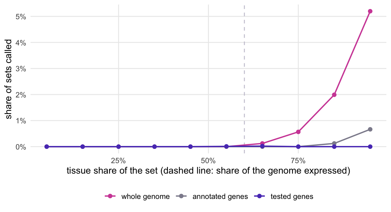
Which sets get called? The next figure pools every set from every experiment and shows how often sets were called, against their tissue share.
brks <-seq(0, 1, by =0.1)per_set$bin <-cut(per_set$tissue, brks, include.lowest =TRUE)mid <- (head(brks, -1) +tail(brks, -1)) /2rate <-do.call(rbind, lapply(names(uni_lab), function(u) { r <-tapply(per_set[[u]], per_set$bin, mean)data.frame(mid = mid, rate =as.numeric(r), background = uni_lab[[u]])}))rate <- rate[!is.na(rate$rate), ]rate$background <-factor(rate$background, levels = uni_lab)ggplot(rate, aes(mid, rate, colour = background)) +geom_vline(xintercept = share_expr, linetype ="dashed", colour ="#c9c7d4") +geom_line(linewidth =0.8) +geom_point(size =2) +scale_colour_manual(values =setNames(uni_col, uni_lab), name =NULL) +scale_x_continuous(labels =function(x) paste0(100* x, "%")) +scale_y_continuous(labels =function(x) paste0(100* x, "%")) +labs(x ="tissue share of the set (dashed line: share of the genome expressed)",y ="share of sets called") +theme_pc() +theme(legend.position ="bottom")top_bin <-tapply(per_set$genome, per_set$bin, mean)low_max <-max(top_bin[tail(brks, -1) <= share_expr], na.rm =TRUE) # bands at or below etop_bin_ann <-tapply(per_set$annotated, per_set$bin, mean)
Figure 1: How often a gene set was called when no set is enriched, against the share of its members that are expressed in the tissue, pooled over all simulated experiments. Each line is one choice of background.
The false calls come from sets whose members are mostly expressed. With the genome as background, a set in the top band of tissue share (the figure groups sets in bands of 10%) was called in 5.2% of the experiments it appeared in, while not a single set in the bands at or below the genome’s expressed share was called. The annotated background moves the reference point from the expressed share of the genome, 60%, to the expressed share of the annotated genes, 72% on average here, because annotated genes are more often expressed. Only sets above that share are favoured, and less strongly: a set in the top band was called in 0.7% of the experiments. Leaving the universe empty in kegga() or clusterProfiler puts you in this middle row. It is better than the whole genome only because, in this simulation, annotation happens to be tilted towards expressed genes.
The longer the DE list, the more false sets
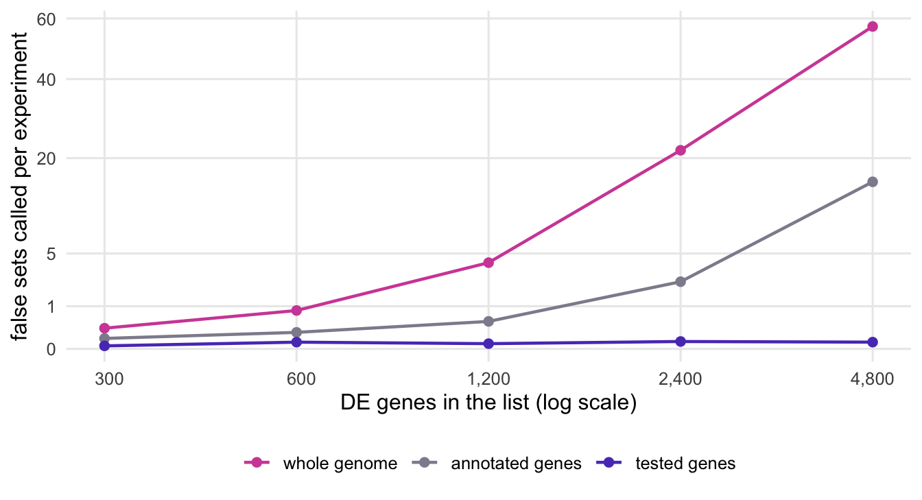
The excess overlap of a mostly expressed set is a fixed ratio, . What changes with the number of DE genes is the power to detect it. The figure repeats the null scenario with DE lists from 300 to 4,800 genes, on the same annotations.
sw <-data.frame(n_de =rep(de_sizes, each =3),calls =as.numeric(sweep[names(uni_lab), ]),background =factor(rep(uni_lab, length(de_sizes)), levels = uni_lab))ggplot(sw, aes(n_de, calls, colour = background)) +geom_line(linewidth =0.8) +geom_point(size =2) +scale_colour_manual(values =setNames(uni_col, uni_lab), name =NULL) +scale_x_continuous(trans ="log2", breaks = de_sizes,labels =function(x) format(x, big.mark =",")) +scale_y_sqrt(breaks =c(0, 1, 5, 20, 40, 60)) +labs(x ="DE genes in the list (log scale)", y ="false sets called per experiment") +theme_pc() +theme(legend.position ="bottom")
Figure 2: Gene sets called per experiment when no set is enriched, against the length of the DE list, for each background. The vertical axis is on a square-root scale.
With 300 DE genes the whole-genome background called 0.23 false sets per experiment; with 4,800 it called 57, and the annotated background 15. The tested background never averaged more than 0.03. So the experiments that look most informative, with strong effects and long DE lists, are the ones that produce the longest lists of tissue terms. It also means that a small pilot study, with its short DE list, can look clean with the wrong background while the full study does not.
A set that is truly enriched
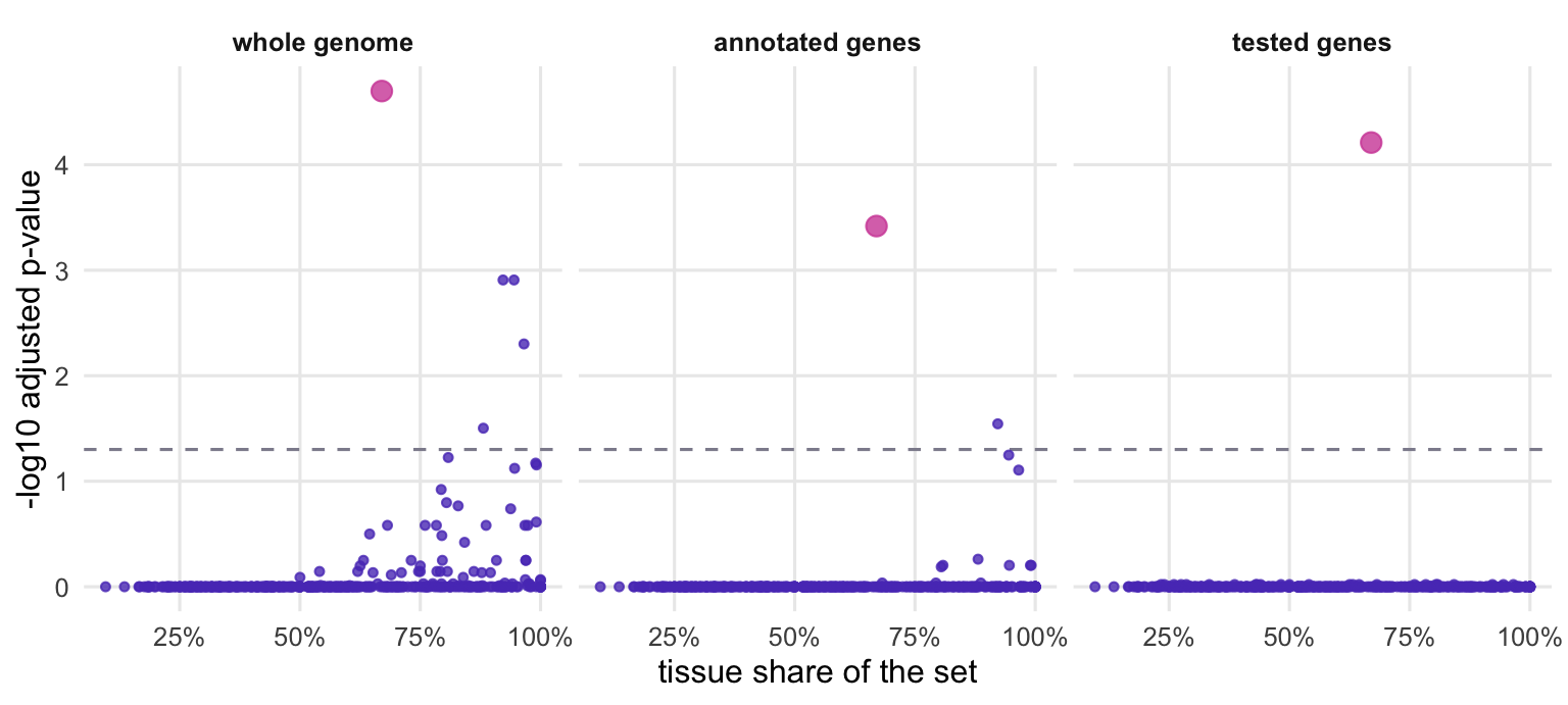
In the second scenario one set holds extra DE genes. The next chunk simulates it, and the figure shows the first of these experiments under each background.
Figure 3: One simulated experiment with a truly enriched set (pink), analysed with three backgrounds. Each point is a gene set; sets above the dashed line are called at the chosen false discovery rate.
In this experiment the whole-genome background called 5 sets, the annotated background 2 and the tested background 1. Over all 200 experiments:
Table 2
background
enriched set called
enriched set ranked first
median p-value of the enriched set
false sets called per experiment
whole genome
76%
48%
1.8e-05
5.17
annotated genes
49%
56%
2.2e-04
0.56
tested genes
66%
86%
1.1e-05
0.06
tested and annotated genes
66%
86%
9.9e-06
0.06
The tested background called the enriched set in 66% of the experiments and ranked it first in 86%, with 0.06 false sets alongside it on average. The whole-genome background called the enriched set more often, in 76% of the experiments, and it is worth seeing why. The set’s own p-value was much the same with either background (the medians are in the table), since its tissue share matches the genome’s. What differs is the correction. The Benjamini-Hochberg procedure compares the -th smallest p-value with times the target rate, where is the number of sets, so every false set that passes lowers the bar for the rest. The enriched set was found more often because it arrived in the company of 5.2 false sets per experiment, and it was ranked first in only 48% of the experiments. Nothing in the output tells you which of the called sets is the real one.
The annotated background shows the opposite failure. It called the enriched set in only 49% of the experiments. The set’s tissue share is below the expressed share of the annotated genes, so this background expects more DE genes in it than the tested background does and penalises it. A wrong background does two things at once: it promotes sets of tissue genes and demotes real signal in sets that are less tissue-specific than average.
Tested is defined by your DE analysis
In the simulation, tested and expressed genes are the same. In real data the tested genes are whatever your DE analysis kept, and each tool keeps a different set. DESeq2 (Love et al. 2014) returns a row for every gene in the count matrix, but not every row was tested. The vignette lists three reasons for missing values: genes with zero counts in every sample get no p-value; genes with an extreme outlier count, detected by Cook’s distance, get no p-value; and genes removed by independent filtering for a low mean count keep their p-value but get no adjusted p-value. None of these genes could be called DE, so none belongs in the background. edgeR and limma-voom remove lowly expressed genes before the fit (Chen et al. 2016), nowadays usually with filterByExpr(), and the tested genes are the rows that remain.
The chunk below simulates a small count matrix, 2,000 genes in 3 against 3 samples, with 60% of genes expressed, and runs both recipes on it.
set.seed(3)n_demo <-2000; n_per_demo <-3group <-factor(rep(c("ctrl", "treat"), each = n_per_demo))expr_demo <-seq_len(n_demo) <= share_expr * n_demomu <-ifelse(expr_demo, exp(rnorm(n_demo, log(40), 1.5)), 0.05) # unexpressed: nearly all zerode_demo <- expr_demo &runif(n_demo) <0.1lfc <-ifelse(de_demo, sample(c(-1.5, 1.5), n_demo, TRUE), 0)mu_mat <- mu *2^outer(lfc, as.numeric(group =="treat"))counts <-matrix(rnbinom(length(mu_mat), mu = mu_mat, size =10), nrow = n_demo,dimnames =list(paste0("gene", seq_len(n_demo)), NULL))# DESeq2: the tested genes are those with an adjusted p-valuedds <-DESeqDataSetFromMatrix(counts, data.frame(group = group), ~ group)dds <-DESeq(dds, quiet =TRUE)res <-results(dds, alpha = fdr_level)universe_deseq <-rownames(res)[!is.na(res$padj)]de_deseq <-rownames(res)[!is.na(res$padj) & res$padj < fdr_level]# edgeR: the tested genes are those kept by filterByExpry <-DGEList(counts, group = group)keep <-filterByExpr(y, group = group)y <-normLibSizes(y[keep, , keep.lib.sizes =FALSE])fit <-glmQLFit(y, model.matrix(~ group), robust =TRUE, legacy =FALSE)tab <-topTags(glmQLFTest(fit, coef =2), n =nrow(y))$tableuniverse_edger <-rownames(y)de_edger <-rownames(tab)[tab$FDR < fdr_level]demo <-c(rows = n_demo, expressed =sum(expr_demo), all_zero =sum(rowSums(counts) ==0),na_p =sum(is.na(res$pvalue)), na_padj_only =sum(!is.na(res$pvalue) &is.na(res$padj)),deseq =length(universe_deseq), edger =length(universe_edger),deseq_unexpr =sum(!expr_demo[match(universe_deseq, rownames(counts))]),edger_unexpr =sum(!expr_demo[match(universe_edger, rownames(counts))]),both =length(intersect(universe_deseq, universe_edger)),de_deseq =length(de_deseq), de_edger =length(de_edger),de_in_u =all(de_deseq %in% universe_deseq) &&all(de_edger %in% universe_edger))stopifnot(demo[["deseq_unexpr"]] ==0, demo[["edger_unexpr"]] ==0, # claims in the text demo[["deseq"]] < demo[["expressed"]], demo[["edger"]] < demo[["expressed"]])
Of the 2,000 rows in DESeq2’s results table, 616 had no p-value, all of them because they had zero counts in every sample, and a further 262 had a p-value but no adjusted p-value, which leaves 1,122 tested genes. filterByExpr() kept 988 genes. Neither background contained an unexpressed gene, but neither contained all 1,200 expressed genes either, and the two backgrounds differ: all 988 genes kept by filterByExpr() are also in DESeq2’s background, which has 134 more. Taking the background from one tool and the DE list from another, or from a separate expression cut-off, mixes two definitions of “tested”.
The DE list should also be a subset of the background. Tools differ in what they do with DE genes that are not in it; limma’s kegga(), for example, drops them without a message (it keeps only the DE genes found in the universe before counting). A one-line check, as in the code below, makes the problem visible instead.
What to do in practice
Take the background and the DE list from the same results table:
# DESeq2: tested genes are those with an adjusted p-valueres <-results(dds, alpha =0.05)universe <-rownames(res)[!is.na(res$padj)]de <-rownames(res)[!is.na(res$padj) & res$padj <0.05]# edgeR or limma-voom: tested genes are the rows left after filterByExpr()# universe <- rownames(y)stopifnot(all(de %in% universe))# limma, with your own gene sets (gene.pathway: gene ID, set ID)kegga(de, universe = universe, gene.pathway = gene_pathway, pathway.names = set_names)# clusterProfiler (not run here)enricher(de, universe = universe, TERM2GENE = term2gene)enrichGO(de, OrgDb = org.Hs.eg.db, keyType ="ENSEMBL", ont ="BP", universe = universe)
The gene identifiers in the background must be of the same type as those in the DE list and the annotation, so convert both with the same mapping.
Two details of the tools are useful to know. kegga() keeps background genes that belong to no set unless you set restrict.universe = TRUE (the default is FALSE). In the simulation the two choices gave practically the same results (compare the last two rows of the first table), so either is fine there.
clusterProfiler intersects the background you give it with the annotated genes. Keep that default. The option options(enrichment_force_universe = TRUE) keeps the unannotated genes in the background, and in DOSE 4.4.0, which runs the test for clusterProfiler 4.18 in Bioconductor 3.22, it does so without adjusting the other side of the table: the number of DE genes drawn is still counted as the DE genes that carry some annotation (n <- rep(length(qExtID2TermID), ...) in enricher_internal()). Every set’s expected overlap is then understated. The chunk below recomputes the null scenario the way DOSE 4.4.0 does, with the tested genes as the universe and enricher()’s default limits on set size (10 to 500 genes).
min_gs <-10; max_gs <-500# enricher() defaults: minGSSize, maxGSSizedose_p <-function(w, is_de, u, force) { ann <- w$universe$annotated bg <-if (force) u else u & ann # background N n <-sum(is_de & ann) # drawn: DE genes with any annotation in_bg <- bg[w$gene] M <-tabulate(w$set[in_bg], n_sets) k <-tabulate(w$set[in_bg & is_de[w$gene]], n_sets) keep <- k >0& M >= min_gs & M <= max_gs # only sets holding a DE gene are testedp.adjust(phyper(k[keep] -1, M[keep], sum(bg) - M[keep], n, lower.tail =FALSE), "BH")}set.seed(4)forced <-t(sapply(seq_len(n_rep), function(r) { w <-make_world() tested <-which(w$expr)unlist(lapply(c(n_de, max(de_sizes)), function(nd) { is_de <-rep(FALSE, n_genes); is_de[sample(tested, nd)] <-TRUEc(default =sum(dose_p(w, is_de, w$universe$tested, FALSE) < fdr_level),force =sum(dose_p(w, is_de, w$universe$tested, TRUE) < fdr_level),share_ann =mean(w$universe$annotated[is_de])) }))}))colnames(forced) <-paste(rep(c("main", "max"), each =3), c("default", "force", "share_ann"), sep ="_")forced_mean <-colMeans(forced)forced_any <-colMeans(forced >0)
With 1,200 DE genes the default called 0.03 sets per experiment and the forced background 0.40, with at least one call in 27.0% of the experiments; with 4,800 DE genes the figures were 0.03 and 28.2. Here 83% of the DE genes were annotated; in real data, where the tested genes include many non-coding genes without GO terms, the share is lower and the inflation larger. The development version of clusterProfiler, which calls enrichit (I read 0.2.5), counts all DE genes in the universe instead, so there the option is harmless. What matters in either case is that the background starts from the tested genes.
# kegga() on the first planted experiment, against the hypergeometric test written abovegene_id <-paste0("g", seq_len(n_genes))gene_pathway <-data.frame(gene = gene_id[ex$w$gene], set =paste0("set", ex$w$set))set_names <-data.frame(set =paste0("set", seq_len(n_sets)), name =paste("set", seq_len(n_sets)))de_ids <- gene_id[ex$is_de]kg_tested <-kegga(de_ids, universe = gene_id[ex$w$expr],gene.pathway = gene_pathway, pathway.names = set_names)kg_default <-kegga(de_ids, gene.pathway = gene_pathway, pathway.names = set_names)i <-match(rownames(kg_tested), set_names$set)diff_tested <-max(abs(kg_tested$P.DE - ex$p[i, "tested"]))i <-match(rownames(kg_default), set_names$set)diff_default <-max(abs(kg_default$P.DE - ex$p[i, "annotated"]))stopifnot(diff_tested <1e-12, diff_default <1e-12)
As a check on the code above, the chunk runs kegga() on the first experiment of the second scenario. With universe set to the tested genes it reproduced the p-values of the tested background, and with no universe those of the annotated background, to within .
When you report an enrichment result, name the background and how it was defined (“all genes with an adjusted p-value in the DESeq2 results table”), so that a reader can judge the list of terms.